As part of recent pipeline development, I’ve had cause to modify and rerun the index workflow several times. This provided an opportunity to (a) parallelise some key bottleneck processes to reduce runtime, and (b) profile cost and resource consumption across processes in the workflow. Here, I present this information for one recent run of the index workflow, which took place overnight on July 16th-17th 2024.
In total, the index workflow ran for a bit under four hours, and consumed a total of 166.6 CPU-hours across processes. According to the AWS Cost Explorer, this run cost $4.74 in compute costs and $1.50 in EBS storage costs, for a total of $6.24, or $0.04 per CPU-hour1.
This is cheaper than I expected! Based on this I feel pretty okay running the index workflow whenever necessary.
Compute
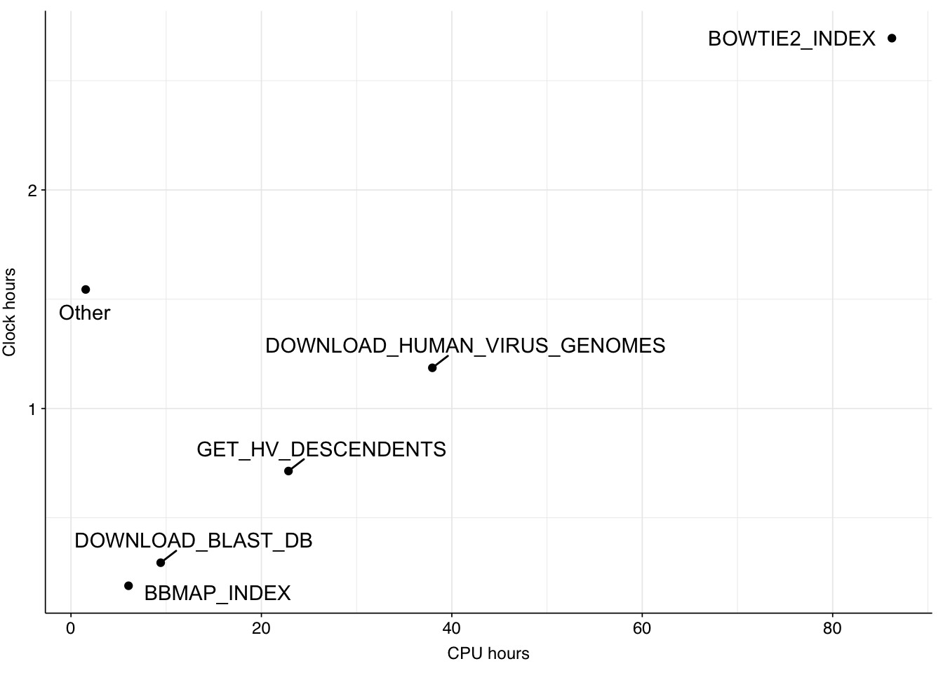
To get a breakdown of the compute spent by the index pipeline, I used nextflow log to get data on the different processes run by the workflow, then calculated the clocktime2 and CPU-hours consumed by each process. The results were as follows:
The CPU-hours of the pipeline are dominated by three processes: constructing Bowtie2 indexes, expanding human-viral taxids to include descendents; and downloading viral genomes for HV index construction. The latter two of these were previously much more costly in terms of clock time but have recently been parallelized, which doesn’t have much effect on CPU-hours but brings clock hours dramatically down.
Conclusion
Overall, the current version of the index workflow is quite cheap in terms of both cost and runtime. Having parallelized a few key bottlenecks, I don’t see obvious low-hanging fruit for further improvement here. As such, I don’t plan to further develop the index workflow unless and until that work is necessitated by changes in other workflow.
Footnotes
This last number matches well with initial data I’ve gathered on costs of the run workflow.↩︎
Note that clock time in the graph is summed across processes that might have been taking place in parallel.↩︎
Source Code
---title: "Profiling the v2 index workflow"subtitle: "Breaking down the computational costs"author: "Will Bradshaw"date: 2024-07-18format: html: code-fold: true code-tools: true code-link: true df-print: pagededitor: visualtitle-block-banner: black---```{r}#| label: preamble#| include: false# Load packageslibrary(tidyverse)library(cowplot)library(patchwork)library(fastqcr)library(RColorBrewer)library(ggpubr)library(ggrepel)source("../scripts/aux_plot-theme.R")# GGplot themes and scalestheme_base <- theme_base +theme(aspect.ratio =NULL)theme_rotate <- theme_base +theme(axis.text.x =element_text(hjust =1, angle =45),)theme_kit <- theme_rotate +theme(axis.title.x =element_blank(),)theme_xblank <- theme_kit +theme(axis.text.x =element_blank())tnl <-theme(legend.position ="none")```As part of recent pipeline development, I've had cause to modify and rerun the index workflow several times. This provided an opportunity to (a) parallelise some key bottleneck processes to reduce runtime, and (b) profile cost and resource consumption across processes in the workflow. Here, I present this information for one recent run of the index workflow, which took place overnight on July 16th-17th 2024.# Cost```{r}# AWS costscost_cpu <-2.81+1.18+0.7+0.05cost_ebs <-0.84+0.4+0.24+0.02cost_total <- cost_cpu + cost_ebscost_cpu_usd <-paste0("$", format(cost_cpu, nsmall=2))cost_ebs_usd <-paste0("$", format(cost_ebs, nsmall=2))cost_total_usd <-paste0("$", format(cost_total, nsmall=2))# Cost per CPU-hourcpu_hours <-166.6cost_per_cpu_hour <- (cost_total/cpu_hours) %>%round(digits=2)cost_per_cpu_hour_usd <-paste0("$", cost_per_cpu_hour)```In total, the index workflow ran for a bit under four hours, and consumed a total of `{r} cpu_hours` CPU-hours across processes. According to the AWS Cost Explorer, this run cost `{r} cost_cpu_usd` in compute costs and `{r} cost_ebs_usd` in EBS storage costs, for a total of `{r} cost_total_usd`, or `{r} cost_per_cpu_hour_usd` per CPU-hour[^1].[^1]: This last number matches well with initial data I've gathered on costs of the run workflow.This is cheaper than I expected! Based on this I feel pretty okay running the index workflow whenever necessary.# ComputeTo get a breakdown of the compute spent by the index pipeline, I used `nextflow log` to get data on the different processes run by the workflow, then calculated the clocktime[^2] and CPU-hours consumed by each process. The results were as follows:[^2]: Note that clock time in the graph is summed across processes that might have been taking place in parallel.```{r}data_dir <-"../data/2024-07-18_index-profiling"log_path <-file.path(data_dir, "log.txt")col_names <-c("process", "cpus", "realtime")log_raw <-read_tsv(log_path, col_names = col_names, show_col_types =FALSE)parse_duration_string <-function(dstr){# Parse an atomic duration string n <-sub("([0-9,.]+).*", "\\1", dstr) %>% as.numeric unit <-sub("[0-9,.]+(.*)", "\\1", dstr)if (unit =="ms") return(n /1000)if (unit =="s") return(n)if (unit =="m") return(n *60)if (unit =="h") return(n *3600)}parse_duration_vector <-function(dvec){# Parse a vector of duration strings dvec %>%sapply(parse_duration_string) %>% sum}parse_durations <-function(durations){# Parse a vector of non-atomic duration strings durations %>%str_split(" ") %>%sapply(parse_duration_vector)}middle <-function(str, sep){ str %>%str_split(sep) %>%sapply(head, -1) %>%sapply(tail, -1) %>%sapply(paste, collapse = sep)}# Parse log datalog <- log_raw %>%mutate(realtime_s =parse_durations(realtime),cpu_hours = realtime_s * cpus /3600,workflow = process %>%str_split(":") %>%sapply(first),job = process %>%str_split(":") %>%sapply(last),subworkflow = process %>%middle(":"))log_summary <- log %>%group_by(job) %>%summarize(cpu_hours =sum(cpu_hours),runtime_hours =sum(realtime_s)/3600) %>%arrange(desc(cpu_hours))log_display <- log_summary %>%mutate(minor = cpu_hours <1,job_display =ifelse(minor, "Other", job)) %>%group_by(job_display) %>%summarize(cpu_hours =sum(cpu_hours),runtime_hours =sum(runtime_hours)) %>%arrange(desc(cpu_hours)) %>%mutate(hjust=-0.05)log_display$hjust[1] <-1.05# Plotg_log <-ggplot(log_display, aes(x=cpu_hours, y=runtime_hours)) +geom_point() +geom_text_repel(aes(label=job_display), box.padding=0.5) +scale_x_continuous(name="CPU hours", breaks =seq(0,200,20)) +scale_y_continuous(name="Clock hours", breaks =seq(0,10,1)) + theme_baseg_log```The CPU-hours of the pipeline are dominated by three processes: constructing Bowtie2 indexes, expanding human-viral taxids to include descendents; and downloading viral genomes for HV index construction. The latter two of these were previously much more costly in terms of clock time but have recently been parallelized, which doesn't have much effect on CPU-hours but brings clock hours dramatically down.# ConclusionOverall, the current version of the index workflow is quite cheap in terms of both cost and runtime. Having parallelized a few key bottlenecks, I don't see obvious low-hanging fruit for further improvement here. As such, I don't plan to further develop the index workflow unless and until that work is necessitated by changes in other workflow.