Continuing my analysis of datasets from the P2RA preprint, I analyzed the data from Brumfield et al. (2022). This study conducted longitudinal monitoring of SARS-CoV-2 via qPCR from a single manhole in Maryland, combined with comprehensive microbiome analysis using metagenomics during a major COVID spike in early 2021. In total, they sequenced six samples from February to April 2021.
One unusual feature that makes this study interesting is that they conducted both RNA and DNA sequencing on each study. Prior to sequencing, samples underwent concentration with the InnovaPrep Concentrating Pipette, followed by separate DNA & RNA extraction using different kits. RNA samples underwent rRNA depletion prior to library prep. All samples were sequenced on an Illumina HiSeq4000 with 2x150bp reads.
The raw data
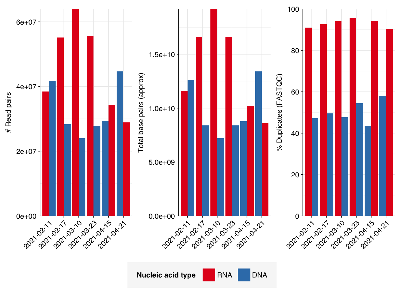
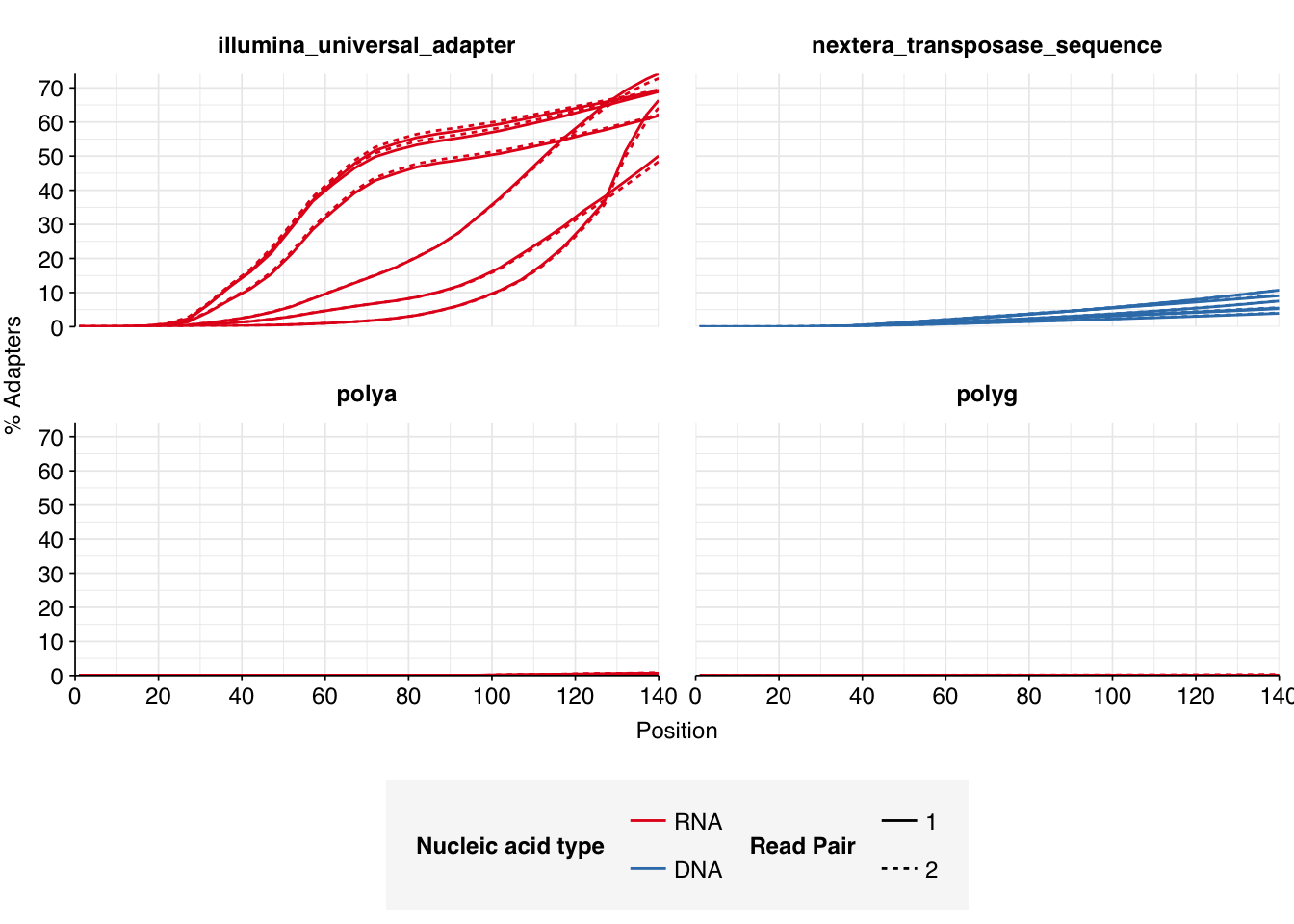
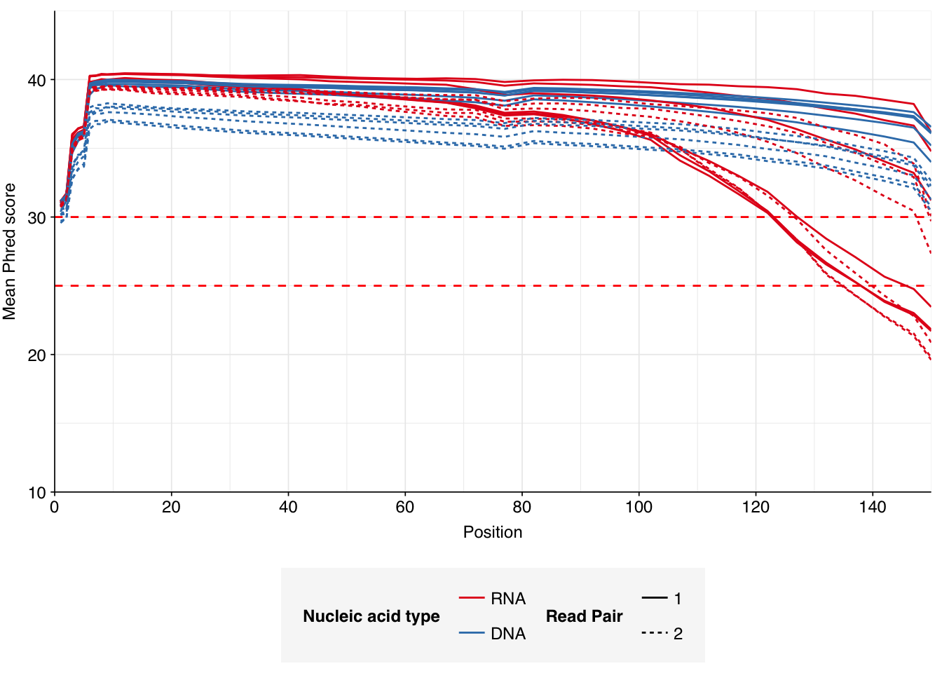
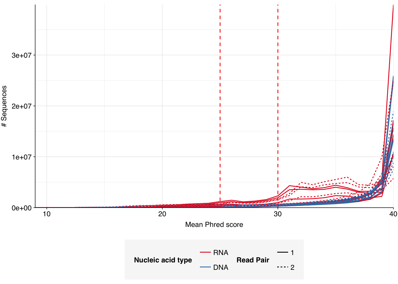
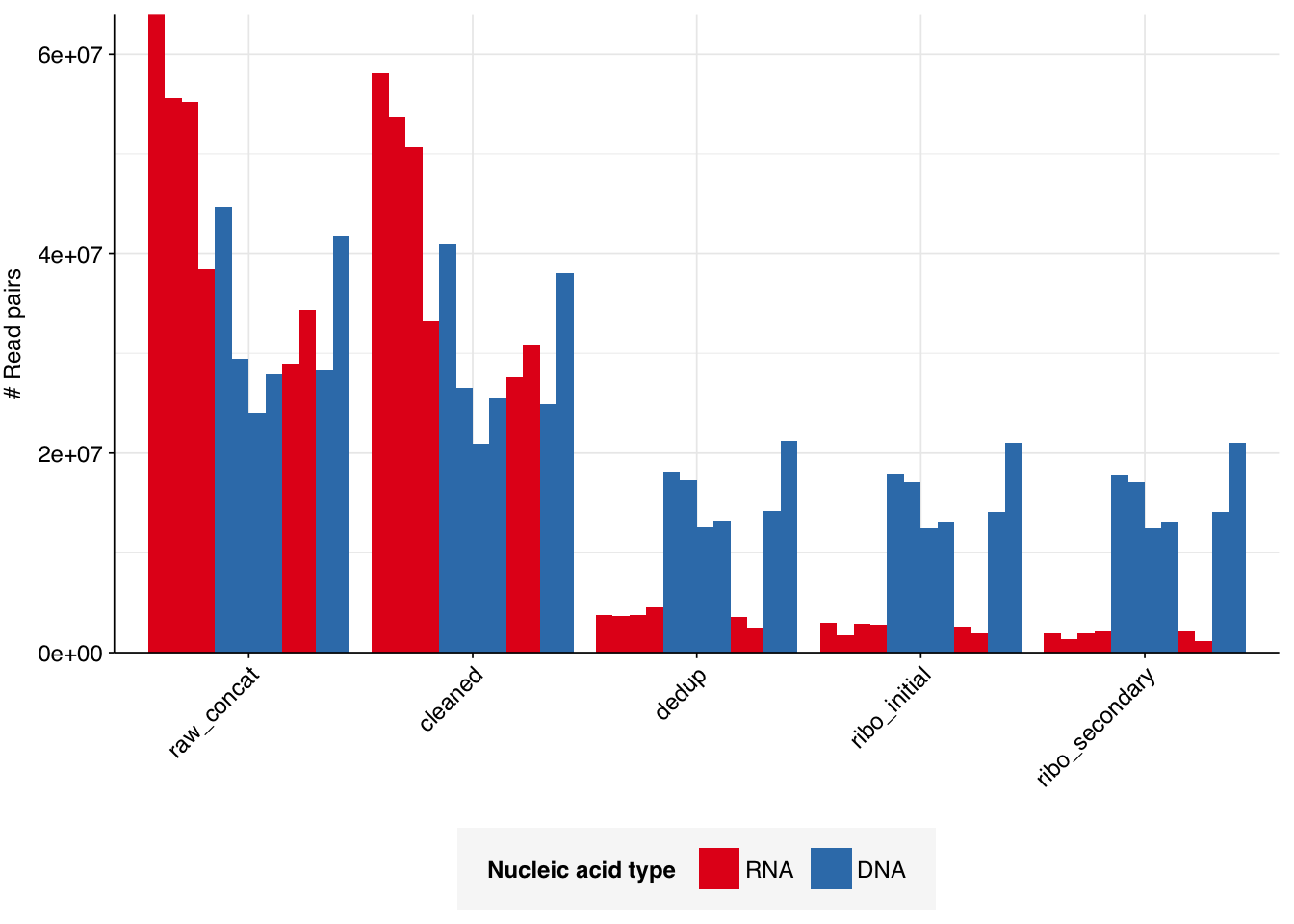
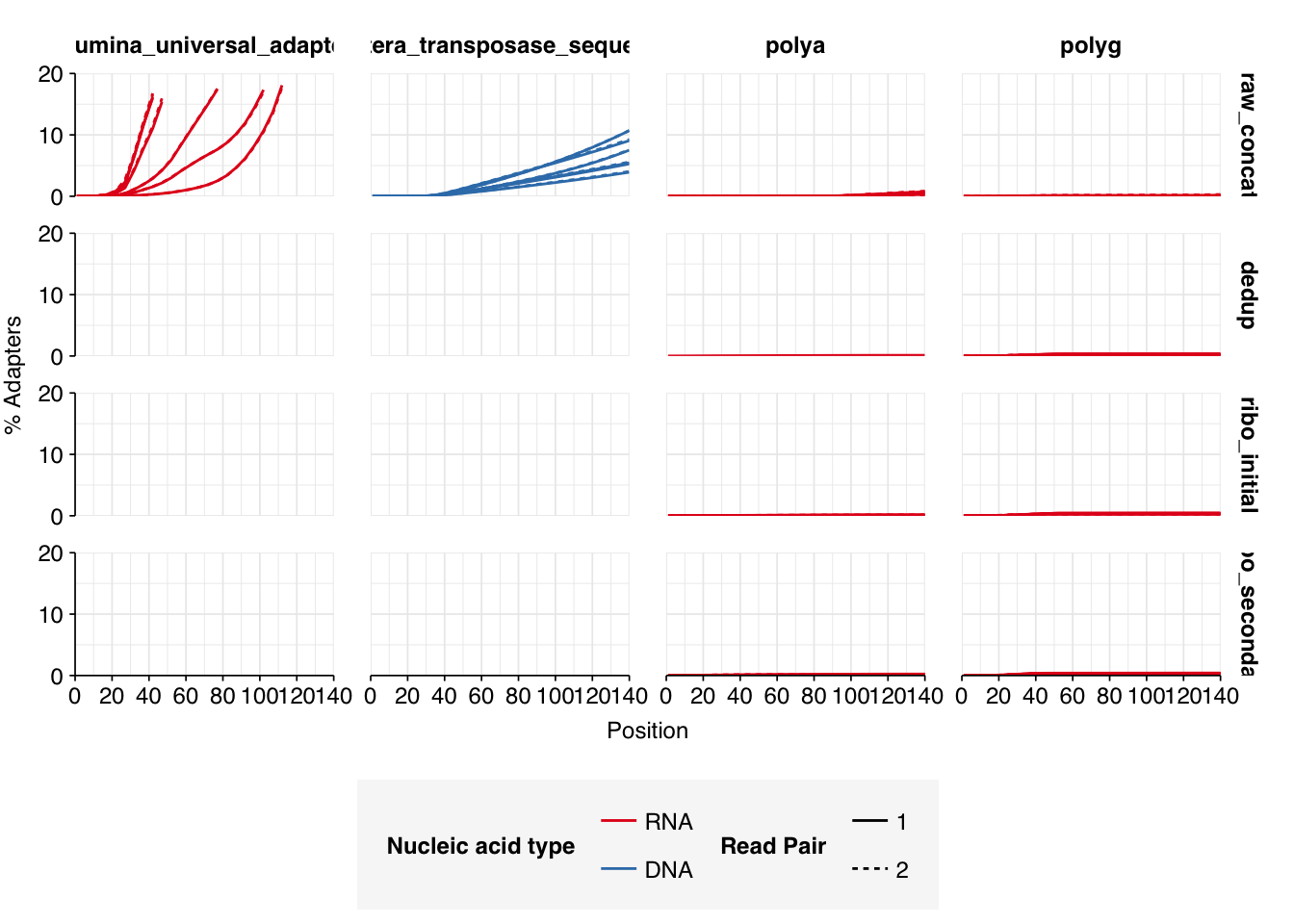
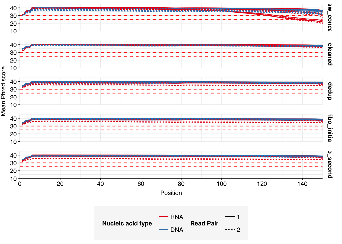
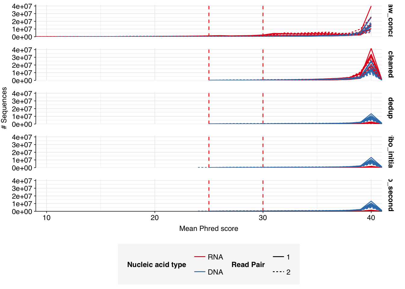
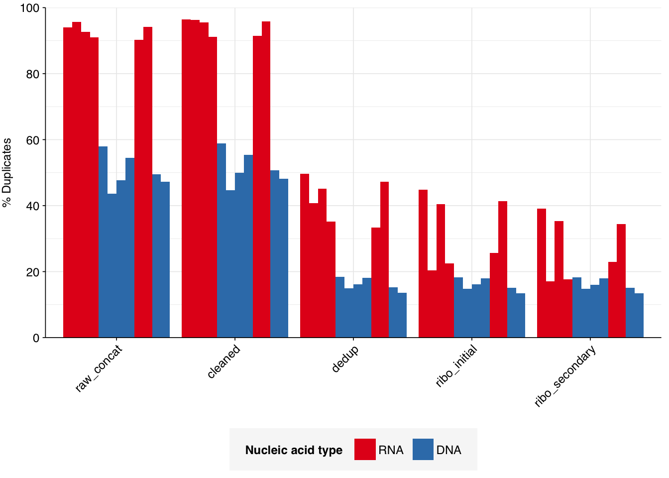
The 6 samples from the Brumfield dataset yielded 24M-45M (mean 33M) DNA-sequencing reads and 29M-64M (mean 46M) RNA-sequencing reads per sample, for a total of 196M DNA read pairs and 276M RNA read pairs (59 and 83 gigabases of sequence, respectively). Read qualities were mostly high but tailed off at the 3’ end in some samples, suggesting the need for trimming. Adapter levels were very high. Inferred duplication levels were 44-58% in DNA reads and 90-96% in RNA reads, i.e. very high.
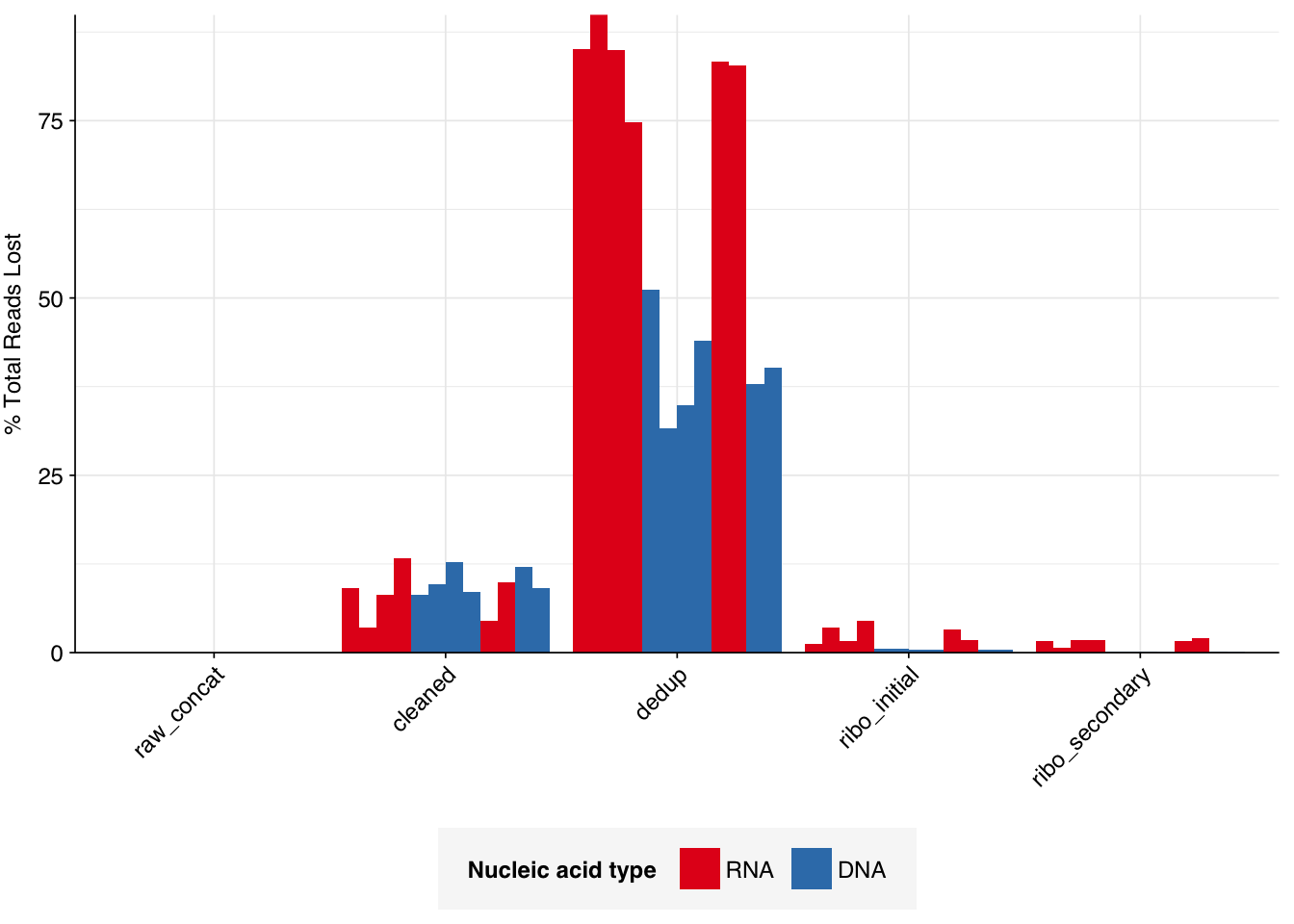
The average fraction of reads lost at each stage in the preprocessing pipeline is shown in the following table. On average, cleaning & deduplication together removed about 50% of total reads from DNA libraries and about 92% from RNA libraries, primarily during deduplication. Only a few reads (low single-digit percentages at most) were lost during subsequent ribodepletion, even in RNA reads, consistent with the samples having undergone rRNA depletion prior to sequencing.
# Plot reads over preprocessingg_reads_stages<-ggplot(basic_stats, aes(x=stage, y=n_read_pairs,fill=na_type,group=sample))+geom_col(position="dodge")+scale_fill_na()+scale_y_continuous("# Read pairs", expand=c(0,0))+theme_kitg_reads_stages
Code
# Plot relative read losses during preprocessingg_reads_rel<-ggplot(n_reads_rel, aes(x=stage, y=p_reads_lost_abs_marginal,fill=na_type,group=sample))+geom_col(position="dodge")+scale_fill_na()+scale_y_continuous("% Total Reads Lost", expand=c(0,0), labels =function(x)x*100)+theme_kitg_reads_rel
Data cleaning with FASTP was very successful at removing adapters, with very few adapter sequences found by FASTQC at any stage after the raw data. FASTP was also successful at improving read quality.
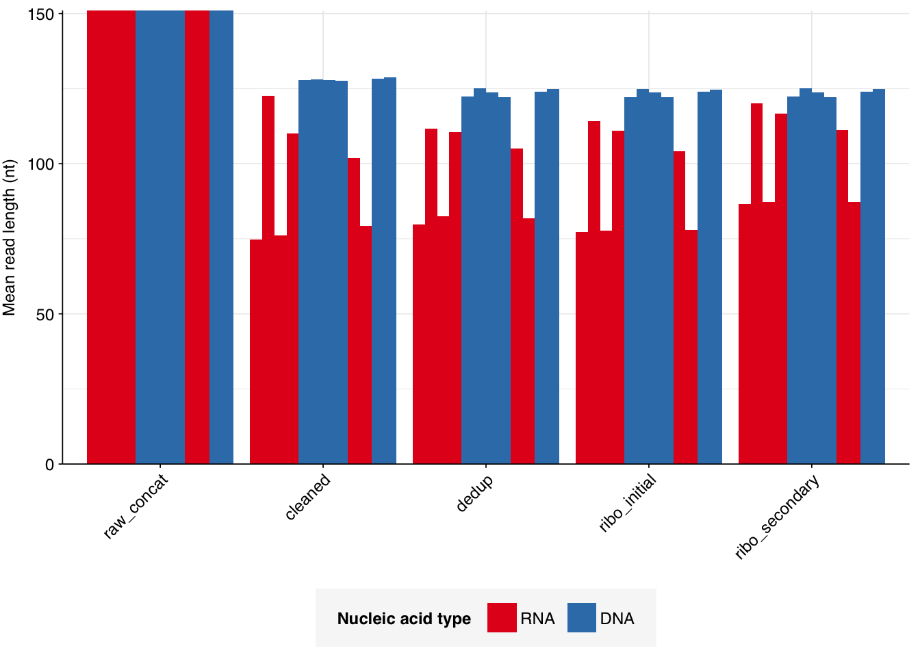
According to FASTQC, deduplication was moderately effective at reducing measured duplicate levels, with FASTQC-measured levels falling from an average of 50% to one of 16% for DNA reads, and from 93% to 42% for RNA reads:
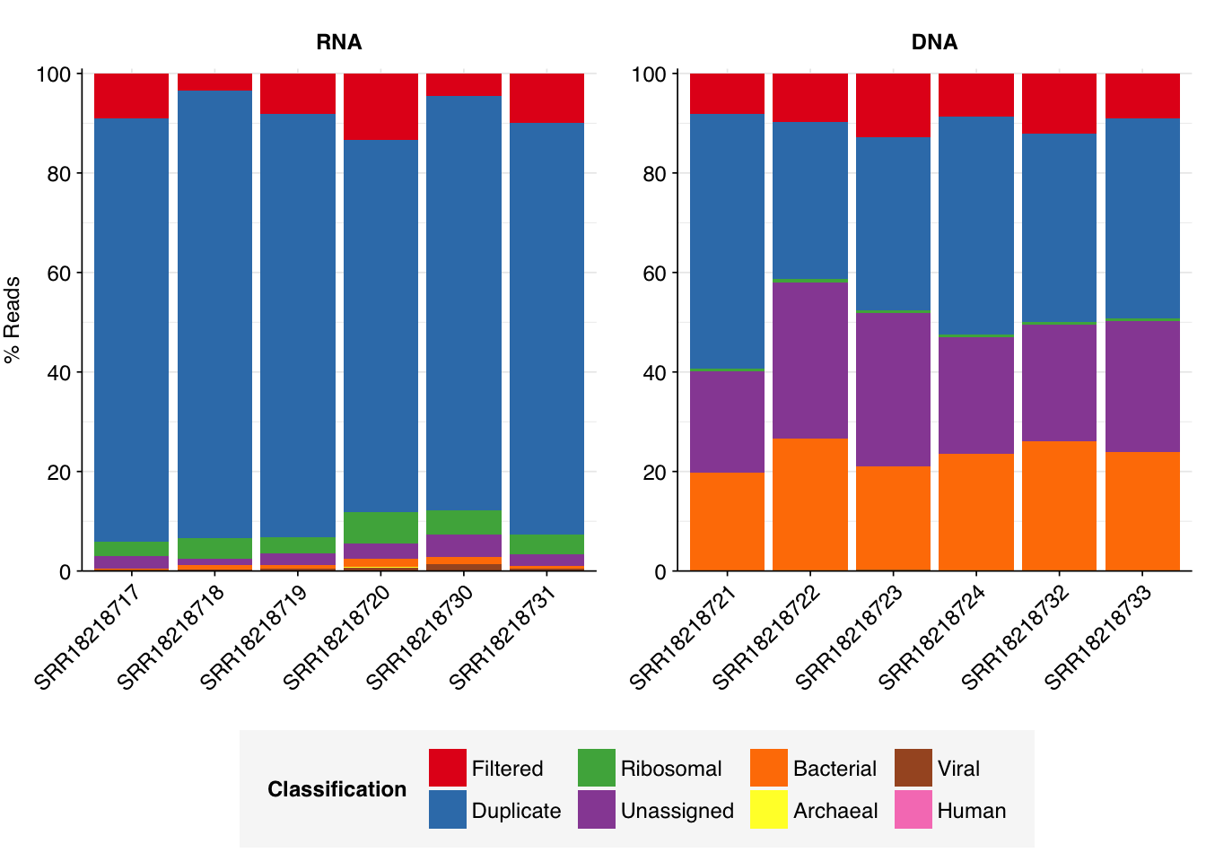
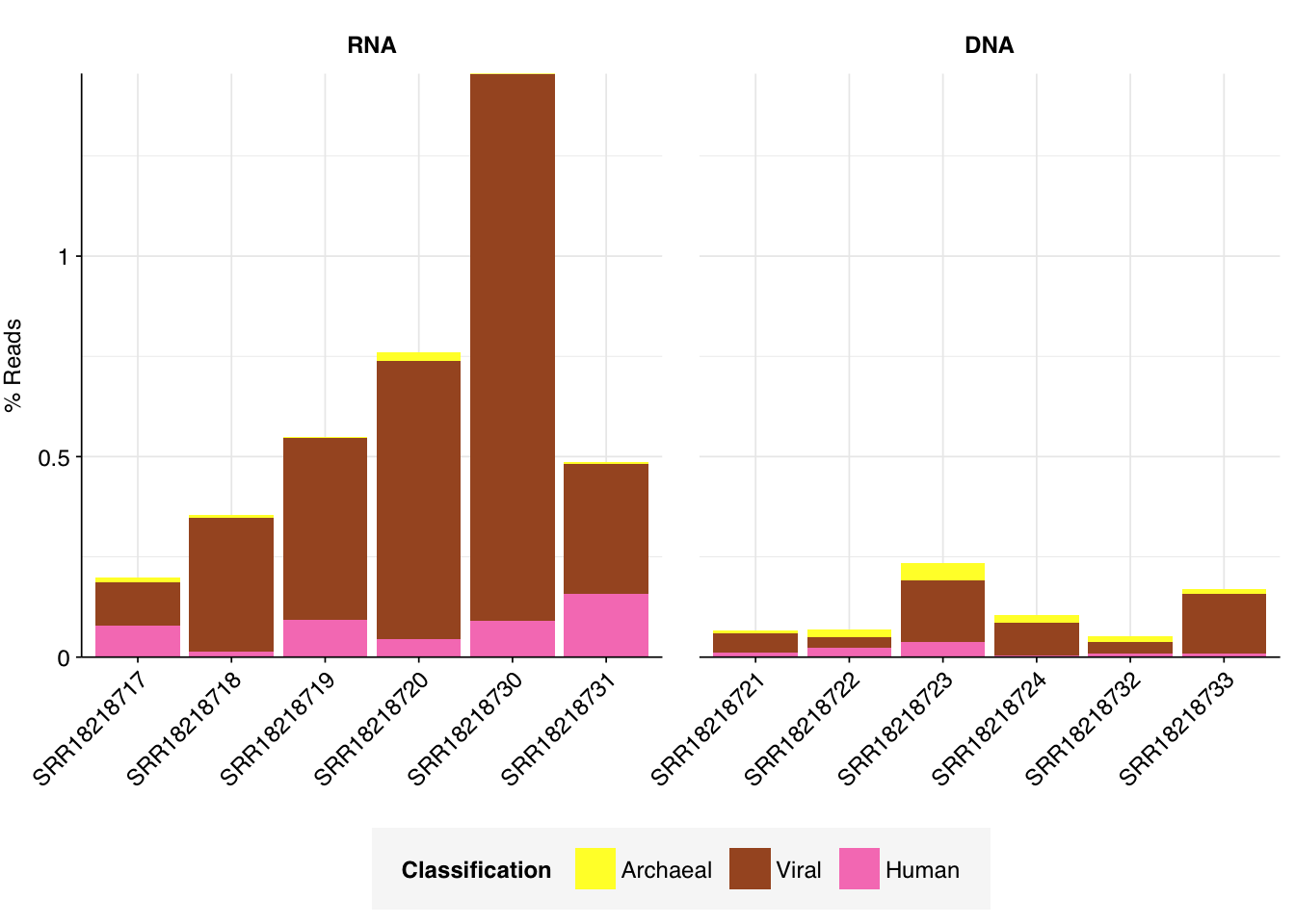
As before, to assess the high-level composition of the reads, I ran the ribodepleted files through Kraken (using the Standard 16 database) and summarized the results with Bracken. Combining these results with the read counts above gives us a breakdown of the inferred composition of the samples:
As previously noted, RNA samples were overwhelmingly composed of duplicates. Despite this, the RNA samples achieved a decently high level of total viral reads, with an average of 0.55% of reads mapping to viruses (higher than Crits-Christoph). Levels of total viral reads were much lower in DNA libraries, which were dominated by unassigned and (non-ribosomal) bacterial sequences.
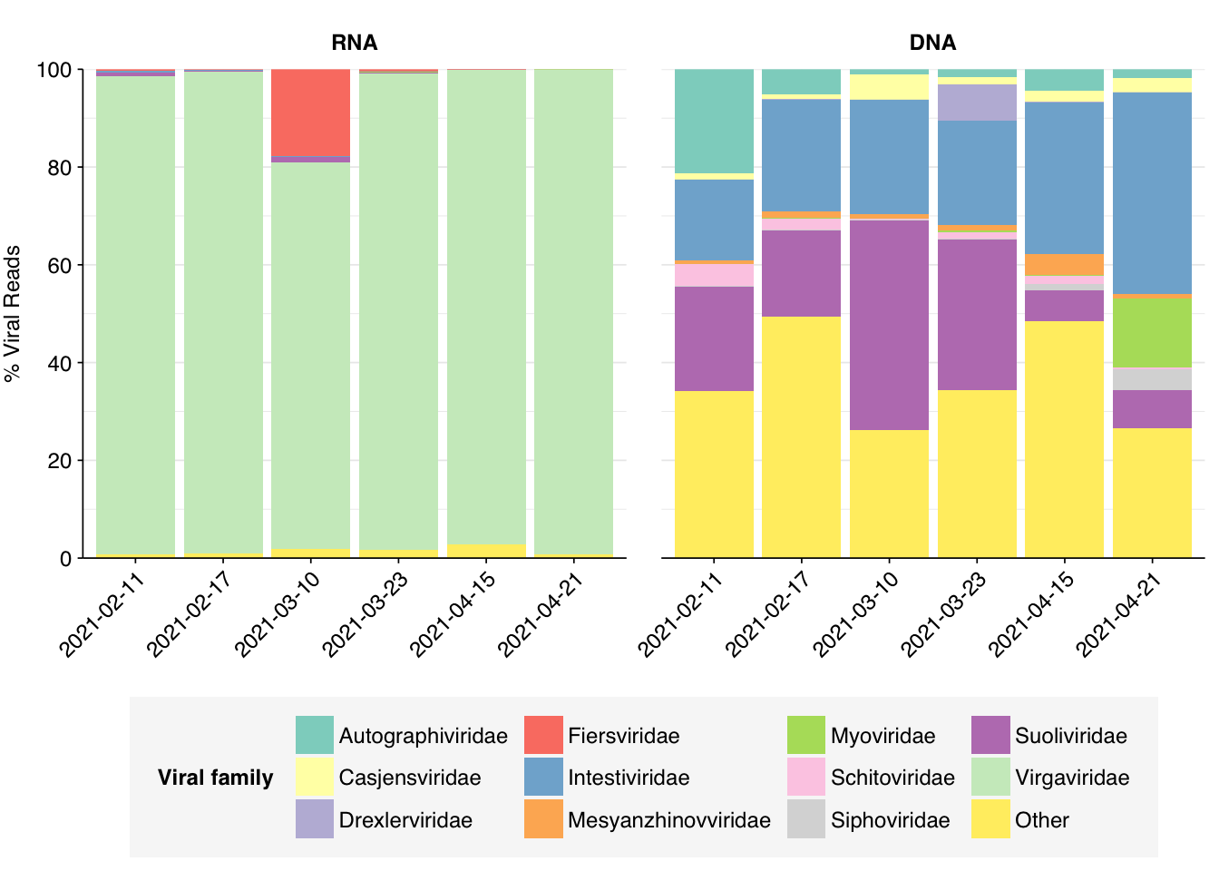
Within viral reads, RNA libraries were (as usual) dominated by plant viruses, particularly Virgaviridae – though one sample, unusually, has a substantial minority of reads from Fiersviridae, a family of RNA phages. Detected DNA viruses come from a wider range of families, but the most abundant families (Suoliviridae, Intestiviridae, Autographiviridae, Myoviridae) are all DNA phages.
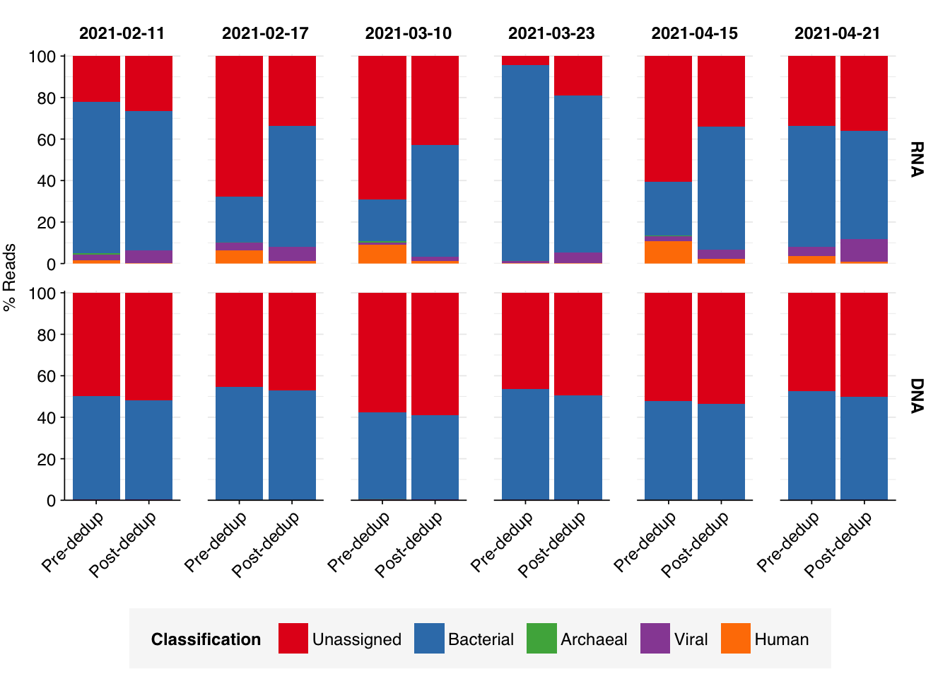
Given the very high level of duplicates in the RNA data, I also repeated the analysis from my second Yang et al. entry, re-running taxonomic composition analysis on pre-deduplication data and comparing the effects of deduplication on composition:
In general, deduplication has little effect on the composition of DNA samples, which remain primarily bacterial and unassigned. A few RNA samples show a reduction in the bacterial (more precisely, bacterial + rRNA) fraction after deduplication, consistent with the presence of some true biological duplicate sequences (most likely rRNA) that are being collapsed. Surprisingly, however, the largest effect is in the opposite direction, with several samples showing large increases in bacterial sequences following deduplication. This suggests that some highly abundant non-bacterial sequence is being collapsed in these samples, increasing the apparent abundance of bacteria.
The increase in bacterial reads in these samples comes at the expense of (1) human reads and (2) the unassigned fraction. The former suggests the presence of human rRNA sequences that are being erroneously incorporated into the post-deduplication “bacterial” fraction; however, this effect is smaller than the decrease in unassigned reads. One possibility might be other non-human eukaryotic rRNA sequences, which Kraken is unable to assign using our current database.
Human-infecting virus reads: validation
Next, I investigated the human-infecting virus read content of these unenriched samples. To get good results here, I needed to make some changes to the pipeline, including adding Trimmomatic as an additional primer-trimming step to prevent further primer-contamination-based false positives. However, for the sake of time I’m not describing them in detail here; if you want to see more I encourage you to check the commit log at the workflow repo.
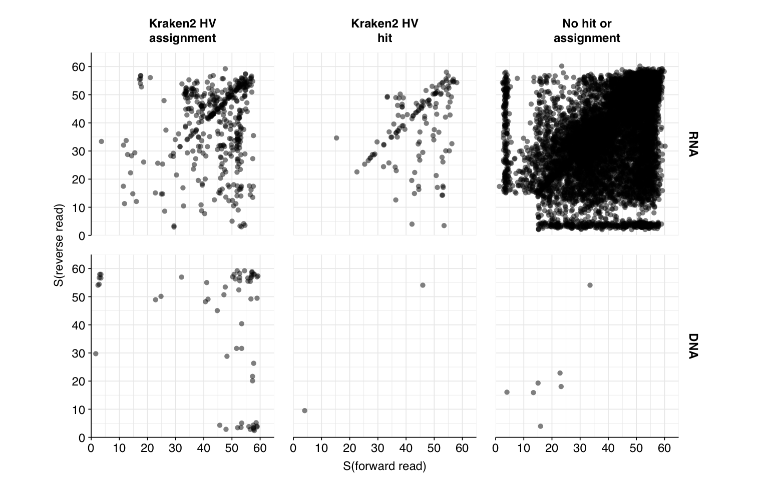
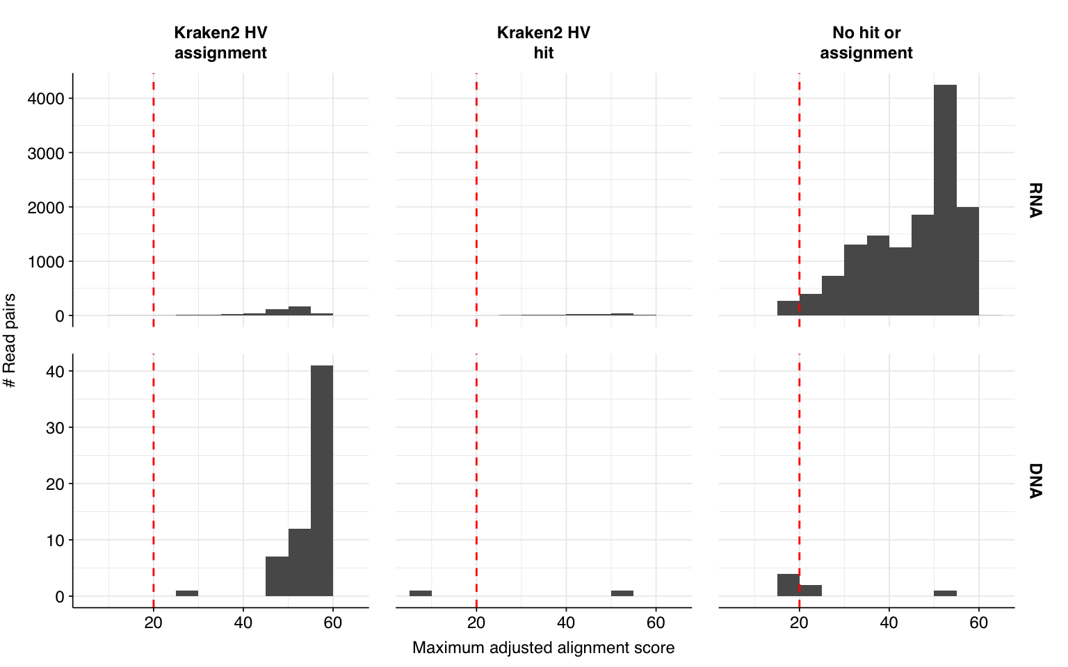
Having made these changes, the workflow identified a total of 14,073 RNA read pairs and 70 DNA read pairs across all samples (0.09% and 0.00009% of surviving reads, respectively).
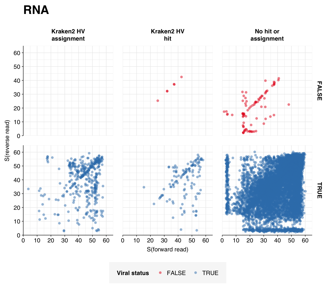
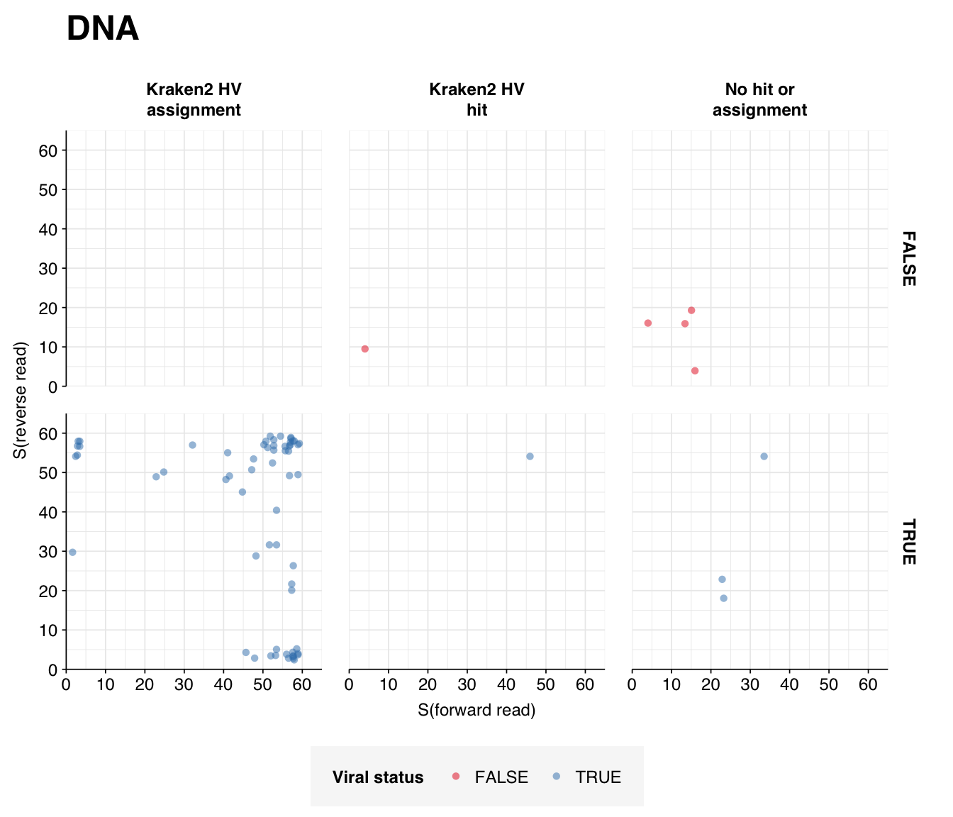
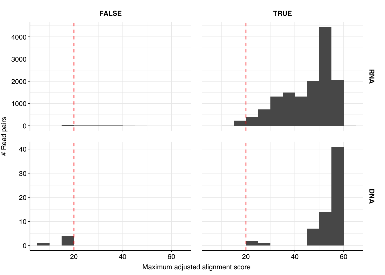
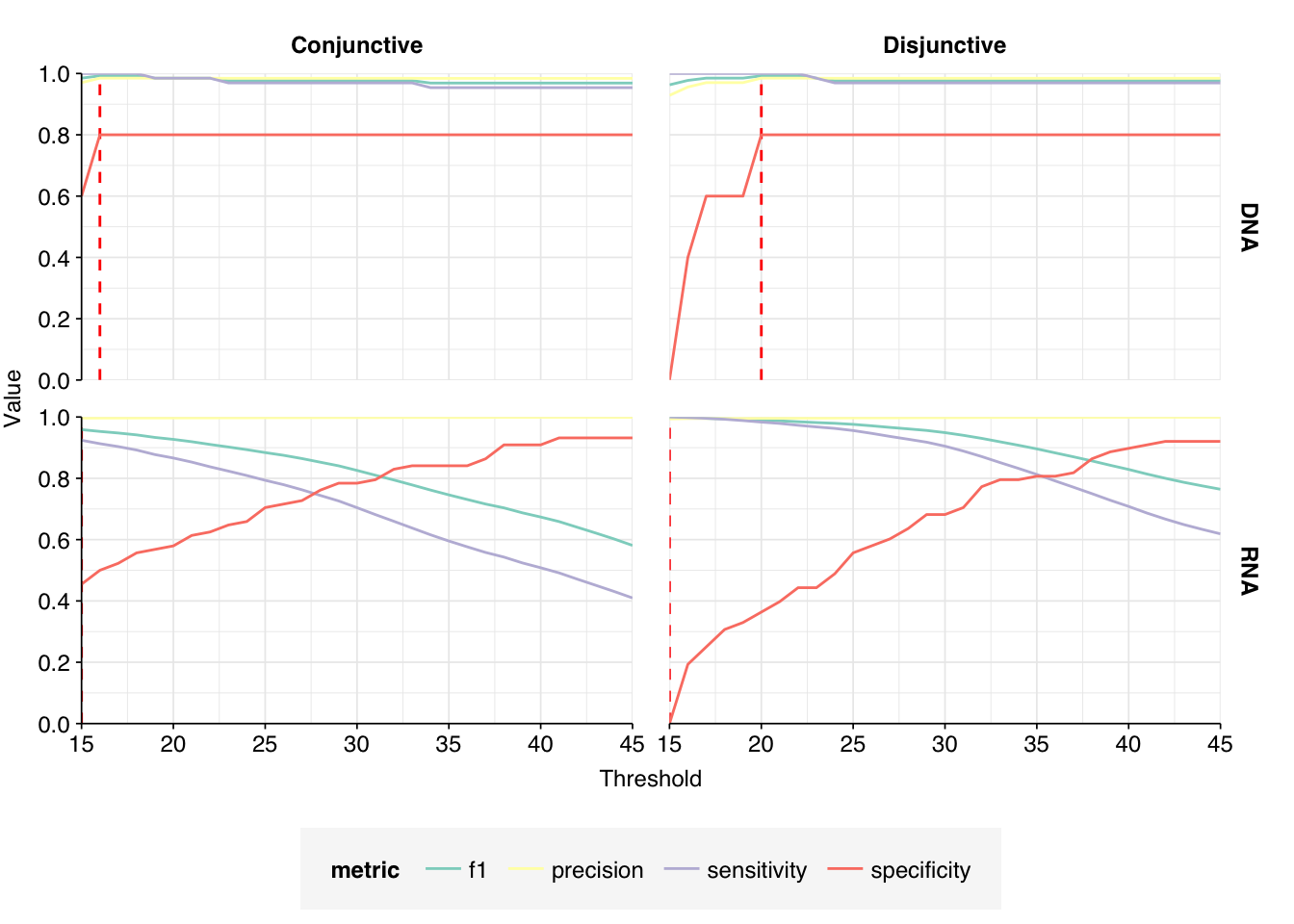
These results look very good on visual inspection, and indeed precision and sensitivity are both very high. For a disjunctive score threshold of 20, my updated workflow achieves an F1 score of 99.0% for RNA sequences and 99.2% for DNA sequences; more than high enough to continue on to human viral analysis.
# Get raw read countsread_counts_raw<-basic_stats_raw%>%select(sample, date, na_type, n_reads_raw =n_read_pairs)# Get HV read countsmrg_hv<-mrg%>%mutate(hv_status =assigned_hv|hit_hv|adj_score_max>=20)read_counts_hv<-mrg_hv%>%filter(hv_status)%>%group_by(sample)%>%count(name="n_reads_hv")read_counts<-read_counts_raw%>%left_join(read_counts_hv, by="sample")%>%mutate(n_reads_hv =replace_na(n_reads_hv, 0))# Aggregateread_counts_total<-read_counts%>%group_by(na_type)%>%summarize(n_reads_raw =sum(n_reads_raw), n_reads_hv =sum(n_reads_hv))%>%mutate(sample="All samples", date ="All dates")read_counts_agg<-read_counts%>%arrange(date)%>%mutate(date =as.character(date))%>%arrange(sample)%>%bind_rows(read_counts_total)%>%mutate(sample =fct_inorder(sample), date =fct_inorder(date), p_reads_hv =n_reads_hv/n_reads_raw)# Get old countsn_hv_reads_old<-c(691, 121, 18, 224, 2, 26, 6, 21, 4, 29, 12, 22)n_hv_reads_old[13]<-sum(n_hv_reads_old[which(read_counts$na_type=="RNA")])n_hv_reads_old[14]<-sum(n_hv_reads_old[which(read_counts$na_type=="DNA")])read_counts_comp<-read_counts_agg%>%mutate(n_reads_hv_old =n_hv_reads_old, p_reads_hv_old =n_reads_hv_old/n_reads_raw)
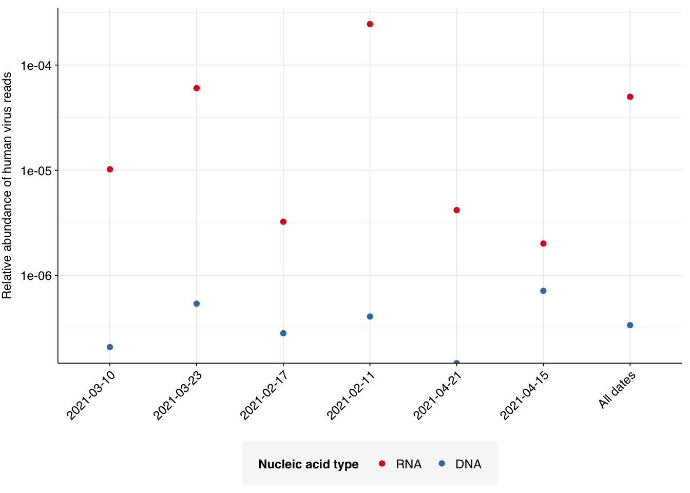
Applying a disjunctive cutoff at S=20 identifies 13,809 RNA reads and 66 DNA reads as human-viral. This gives an overall relative HV abundance of \(5.00 \times 10^{-5}\) for RNA reads and \(3.66 \times 10^{-7}\) for DNA reads. In contrast, the overall HV in the public dashboard is \(3.93 \times 10^{-6}\) for RNA reads and \(4.54 \times 10^{-7}\); the measured HV has thus increased 12.7x for RNA reads, but decreased slightly for DNA reads.
Code
# Visualizeg_phv_agg<-ggplot(read_counts_agg, aes(x=date, color=na_type))+geom_point(aes(y=p_reads_hv))+scale_y_log10("Relative abundance of human virus reads")+scale_color_na()+theme_kitg_phv_agg
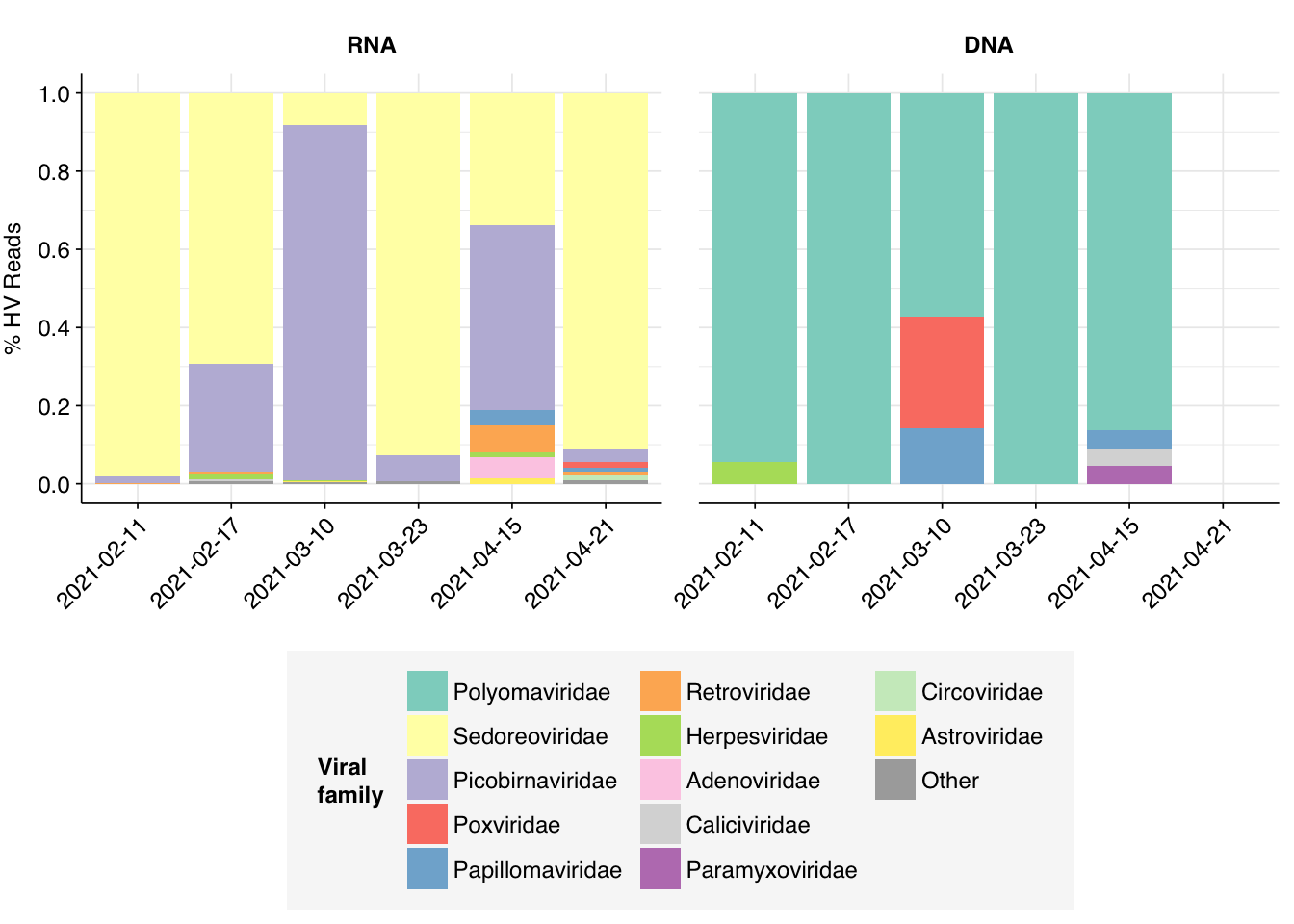
Digging into individual viruses, we see that fecal-oral viruses predominate, especially Mamastrovirus, Rotavirus, Salivirus, and fecal-oral Enterovirus species (especially Enterovirus C, which includes poliovirus):
Code
# Get viral taxon names for putative HV readsviral_taxa$name[viral_taxa$taxid==249588]<-"Mamastrovirus"viral_taxa$name[viral_taxa$taxid==194960]<-"Kobuvirus"viral_taxa$name[viral_taxa$taxid==688449]<-"Salivirus"viral_taxa$name[viral_taxa$taxid==585893]<-"Picobirnaviridae"viral_taxa$name[viral_taxa$taxid==333922]<-"Betapapillomavirus"viral_taxa$name[viral_taxa$taxid==334207]<-"Betapapillomavirus 3"viral_taxa$name[viral_taxa$taxid==369960]<-"Porcine type-C oncovirus"viral_taxa$name[viral_taxa$taxid==333924]<-"Betapapillomavirus 2"mrg_hv_named<-mrg_hv%>%left_join(viral_taxa, by="taxid")# Discover viral species & genera for HV readsraise_rank<-function(read_db, taxid_db, out_rank="species", verbose=FALSE){# Get higher ranks than search rankranks<-c("subspecies", "species", "subgenus", "genus", "subfamily", "family", "suborder", "order", "class", "subphylum", "phylum", "kingdom", "superkingdom")rank_match<-which.max(ranks==out_rank)high_ranks<-ranks[rank_match:length(ranks)]# Merge read DB and taxid DBreads<-read_db%>%select(-parent_taxid, -rank, -name)%>%left_join(taxid_db, by="taxid")# Extract sequences that are already at appropriate rankreads_rank<-filter(reads, rank==out_rank)# Drop sequences at a higher rank and return unclassified sequencesreads_norank<-reads%>%filter(rank!=out_rank, !rank%in%high_ranks, !is.na(taxid))while(nrow(reads_norank)>0){# As long as there are unclassified sequences...# Promote read taxids and re-merge with taxid DB, then re-classify and filterreads_remaining<-reads_norank%>%mutate(taxid =parent_taxid)%>%select(-parent_taxid, -rank, -name)%>%left_join(taxid_db, by="taxid")reads_rank<-reads_remaining%>%filter(rank==out_rank)%>%bind_rows(reads_rank)reads_norank<-reads_remaining%>%filter(rank!=out_rank, !rank%in%high_ranks, !is.na(taxid))}# Finally, extract and append reads that were excluded during the processreads_dropped<-reads%>%filter(!seq_id%in%reads_rank$seq_id)reads_out<-reads_rank%>%bind_rows(reads_dropped)%>%select(-parent_taxid, -rank, -name)%>%left_join(taxid_db, by="taxid")return(reads_out)}hv_reads_species<-raise_rank(mrg_hv_named, viral_taxa, "species")hv_reads_genus<-raise_rank(mrg_hv_named, viral_taxa, "genus")hv_reads_family<-raise_rank(mrg_hv_named, viral_taxa, "family")
Code
# Count reads for each human-viral familyhv_family_counts<-hv_reads_family%>%group_by(sample, date, na_type, name, taxid)%>%count(name ="n_reads_hv")%>%group_by(sample, date, na_type)%>%mutate(p_reads_hv =n_reads_hv/sum(n_reads_hv))# Identify high-ranking families and group othershv_family_major_tab<-hv_family_counts%>%group_by(name)%>%filter(p_reads_hv==max(p_reads_hv))%>%filter(row_number()==1)%>%arrange(desc(p_reads_hv))%>%filter(p_reads_hv>0.01)hv_family_counts_major<-hv_family_counts%>%mutate(name_display =ifelse(name%in%hv_family_major_tab$name, name, "Other"))%>%group_by(sample, date, na_type, name_display)%>%summarize(n_reads_hv =sum(n_reads_hv), p_reads_hv =sum(p_reads_hv), .groups="drop")%>%mutate(name_display =factor(name_display, levels =c(hv_family_major_tab$name, "Other")))# Plot family compositionpalette<-c(brewer.pal(12, "Set3"), "#AAAAAA")g_hv_families<-ggplot(hv_family_counts_major, aes(x=date, y=p_reads_hv, fill=name_display))+geom_col(position="stack")+scale_fill_manual(name="Viral\nfamily", values=palette)+scale_y_continuous(name="% HV Reads", limits=c(0,1), breaks=seq(0,1,0.2))+facet_grid(.~na_type)+guides(fill=guide_legend(ncol=3))+theme_kitg_hv_families
Code
# Count reads for each human-viral genushv_genus_counts<-hv_reads_genus%>%group_by(sample, date, na_type, name, taxid)%>%count(name ="n_reads_hv")%>%group_by(sample, date, na_type)%>%mutate(p_reads_hv =n_reads_hv/sum(n_reads_hv))# Identify high-ranking genera and group othershv_genus_major_tab<-hv_genus_counts%>%group_by(name)%>%filter(p_reads_hv==max(p_reads_hv))%>%filter(row_number()==1)%>%arrange(desc(p_reads_hv))%>%filter(p_reads_hv>0.02)hv_genus_counts_major<-hv_genus_counts%>%mutate(name_display =ifelse(name%in%hv_genus_major_tab$name, name, "Other"))%>%group_by(sample, date, na_type, name_display)%>%summarize(n_reads_hv =sum(n_reads_hv), p_reads_hv =sum(p_reads_hv), .groups="drop")%>%mutate(name_display =factor(name_display, levels =c(hv_genus_major_tab$name, "Other")))# Plot genus compositionpalette<-c(brewer.pal(12, "Set3"), "#AAAAAA")g_hv_genera<-ggplot(hv_genus_counts_major, aes(x=date, y=p_reads_hv, fill=name_display))+geom_col(position="stack")+scale_fill_manual(name="Viral\ngenus", values=palette)+scale_y_continuous(name="% HV Reads", limits=c(0,1), breaks=seq(0,1,0.2))+facet_grid(.~na_type)+guides(fill=guide_legend(ncol=3))+theme_kitg_hv_genera
Code
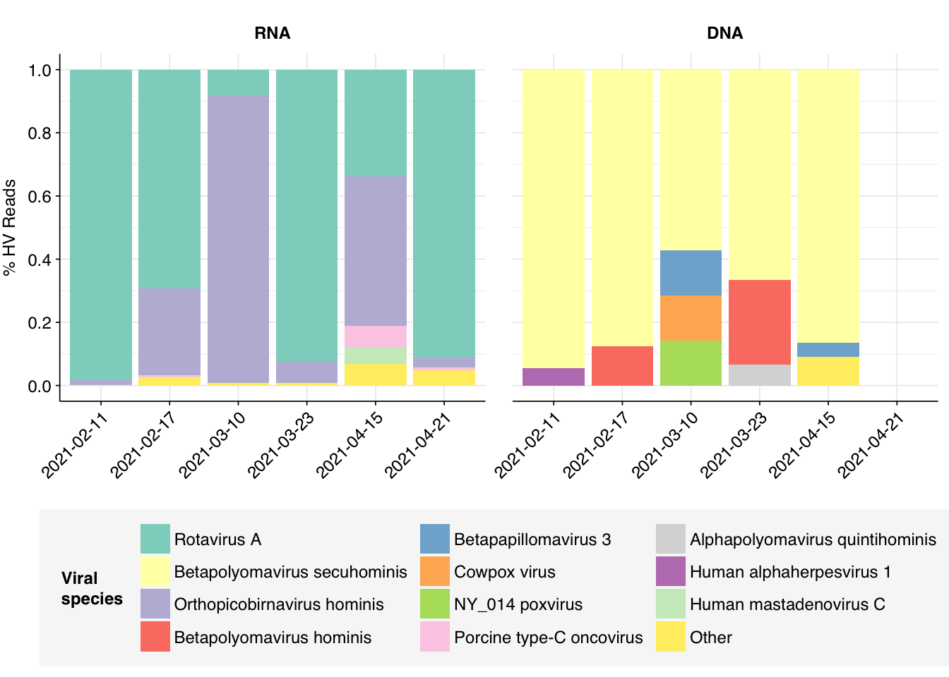
# Count reads for each human-viral specieshv_species_counts<-hv_reads_species%>%group_by(sample, date, na_type, name, taxid)%>%count(name ="n_reads_hv")%>%group_by(sample, date, na_type)%>%mutate(p_reads_hv =n_reads_hv/sum(n_reads_hv))# Identify high-ranking species and group othershv_species_major_tab<-hv_species_counts%>%group_by(name, taxid)%>%filter(p_reads_hv==max(p_reads_hv))%>%filter(row_number()==1)%>%arrange(desc(p_reads_hv))%>%filter(p_reads_hv>0.05)hv_species_counts_major<-hv_species_counts%>%mutate(name_display =ifelse(name%in%hv_species_major_tab$name, name, "Other"))%>%group_by(sample, date, na_type, name_display)%>%summarize(n_reads_hv =sum(n_reads_hv), p_reads_hv =sum(p_reads_hv), .groups="drop")%>%mutate(name_display =factor(name_display, levels =c(hv_species_major_tab$name, "Other")))# Plot species compositionpalette<-c(brewer.pal(12, "Set3"), "#AAAAAA")g_hv_species<-ggplot(hv_species_counts_major, aes(x=date, y=p_reads_hv, fill=name_display))+geom_col(position="stack")+scale_fill_manual(name="Viral\nspecies", values=palette)+scale_y_continuous(name="% HV Reads", limits=c(0,1), breaks=seq(0,1,0.2))+facet_grid(.~na_type)+guides(fill=guide_legend(ncol=3))+theme_kitg_hv_species
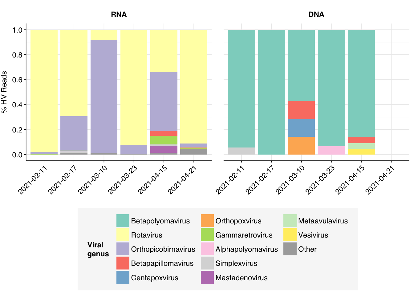
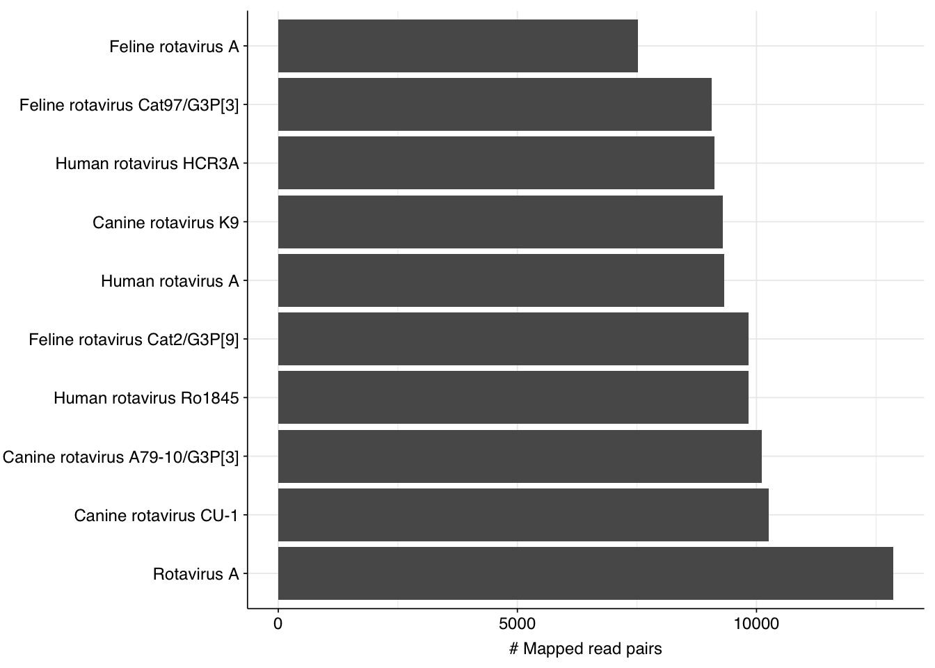
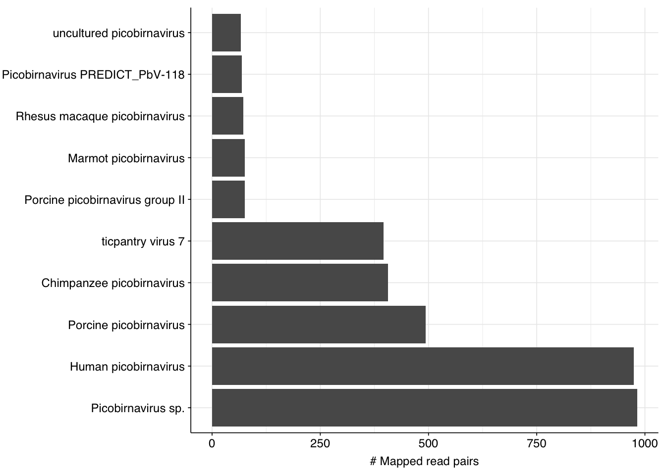
By far the most common virus according to my pipeline (with over 91% of human-viral reads) is Rotavirus A; second (with 8%) is Orthopicobirnavirus hominis. Together, these two enteric RNA viruses dominate HV RNA reads in all samples. Both appear to be real; at least, BLASTN primarily maps these reads to the same or closely-related viruses to that identified by Bowtie2:
I’m quite happy with the quality of the human-viral selection process for this dataset, which ended up achieving very high precision and sensitivity. The most striking result coming out of this analysis is probably the drastic difference in total HV abundance between RNA and DNA reads, with the former >100x higher despite very similar processing methods. In the past we’ve attributed low HV abundance in the DNA datasets we’ve analyzed to the lack of viral enrichment in available DNA datasets; in this case, however, there is very little difference between the DNA and RNA processing methods, so this explanation doesn’t really hold. This makes me more pessimistic about achieving good HV relative abundance with DNA sequencing, even with improved viral enrichment methods.
Source Code
---title: "Workflow analysis of Brumfield et al. (2022)"subtitle: "Wastewater from a manhole in Maryland."author: "Will Bradshaw"date: 2024-04-08format: html: code-fold: true code-tools: true code-link: true df-print: pagededitor: visualtitle-block-banner: black---```{r}#| label: load-packages#| include: falselibrary(tidyverse)library(cowplot)library(patchwork)library(fastqcr)library(RColorBrewer)source("../scripts/aux_plot-theme.R")theme_base <- theme_base +theme(aspect.ratio =NULL)theme_kit <- theme_base +theme(axis.text.x =element_text(hjust =1, angle =45),axis.title.x =element_blank(),)tnl <-theme(legend.position ="none")```Continuing my analysis of datasets from the [P2RA preprint](https://doi.org/10.1101/2023.12.22.23300450), I analyzed the data from [Brumfield et al. (2022)](https://doi.org/10.1128/mbio.00591-22). This study conducted longitudinal monitoring of SARS-CoV-2 via qPCR from a single manhole in Maryland, combined with comprehensive microbiome analysis using metagenomics during a major COVID spike in early 2021. In total, they sequenced six samples from February to April 2021.One unusual feature that makes this study interesting is that they conducted both RNA and DNA sequencing on each study. Prior to sequencing, samples underwent concentration with the InnovaPrep Concentrating Pipette, followed by separate DNA & RNA extraction using different kits. RNA samples underwent rRNA depletion prior to library prep. All samples were sequenced on an Illumina HiSeq4000 with 2x150bp reads.# The raw dataThe 6 samples from the Brumfield dataset yielded 24M-45M (mean 33M) DNA-sequencing reads and 29M-64M (mean 46M) RNA-sequencing reads per sample, for a total of 196M DNA read pairs and 276M RNA read pairs (59 and 83 gigabases of sequence, respectively). Read qualities were mostly high but tailed off at the 3' end in some samples, suggesting the need for trimming. Adapter levels were very high. Inferred duplication levels were 44-58% in DNA reads and 90-96% in RNA reads, i.e. very high.```{r}#| warning: false#| label: read-qc-data# Data input pathsdata_dir <-"../data/2024-03-19_brumfield/"libraries_path <-file.path(data_dir, "sample-metadata.csv")basic_stats_path <-file.path(data_dir, "qc_basic_stats.tsv")adapter_stats_path <-file.path(data_dir, "qc_adapter_stats.tsv")quality_base_stats_path <-file.path(data_dir, "qc_quality_base_stats.tsv")quality_seq_stats_path <-file.path(data_dir, "qc_quality_sequence_stats.tsv")# Import libraries and extract metadata from sample nameslibraries <-read_csv(libraries_path, show_col_types =FALSE) %>%arrange(date) %>%mutate(date =fct_inorder(as.character(date))) %>%arrange(desc(na_type)) %>%mutate(na_type =fct_inorder(na_type))# Import QC datastages <-c("raw_concat", "cleaned", "dedup", "ribo_initial", "ribo_secondary")basic_stats <-read_tsv(basic_stats_path, show_col_types =FALSE) %>%inner_join(libraries, by="sample") %>%mutate(stage =factor(stage, levels = stages),sample =fct_inorder(sample))adapter_stats <-read_tsv(adapter_stats_path, show_col_types =FALSE) %>%mutate(sample =sub("_2$", "", sample)) %>%inner_join(libraries, by="sample") %>%mutate(stage =factor(stage, levels = stages),read_pair =fct_inorder(as.character(read_pair)))quality_base_stats <-read_tsv(quality_base_stats_path, show_col_types =FALSE) %>%inner_join(libraries, by="sample") %>%mutate(stage =factor(stage, levels = stages),read_pair =fct_inorder(as.character(read_pair)))quality_seq_stats <-read_tsv(quality_seq_stats_path, show_col_types =FALSE) %>%inner_join(libraries, by="sample") %>%mutate(stage =factor(stage, levels = stages),read_pair =fct_inorder(as.character(read_pair)))# Filter to raw databasic_stats_raw <- basic_stats %>%filter(stage =="raw_concat")adapter_stats_raw <- adapter_stats %>%filter(stage =="raw_concat")quality_base_stats_raw <- quality_base_stats %>%filter(stage =="raw_concat")quality_seq_stats_raw <- quality_seq_stats %>%filter(stage =="raw_concat")``````{r}#| fig-height: 5#| warning: false#| label: plot-basic-stats# Visualize basic statsscale_fill_na <- purrr::partial(scale_fill_brewer, palette="Set1", name="Nucleic acid type")g_basic <-ggplot(basic_stats_raw, aes(x=date, fill=na_type, group=sample)) +scale_fill_na() + theme_kitg_nreads_raw <- g_basic +geom_col(aes(y=n_read_pairs), position ="dodge") +scale_y_continuous(name="# Read pairs", expand=c(0,0))g_nreads_raw_2 <- g_nreads_raw +theme(legend.position ="none")legend_group <-get_legend(g_nreads_raw)g_nbases_raw <- g_basic +geom_col(aes(y=n_bases_approx), position ="dodge") +scale_y_continuous(name="Total base pairs (approx)", expand=c(0,0)) +theme(legend.position ="none")g_ndup_raw <- g_basic +geom_col(aes(y=percent_duplicates), position ="dodge") +scale_y_continuous(name="% Duplicates (FASTQC)", expand=c(0,0), limits =c(0,100), breaks =seq(0,100,20)) +theme(legend.position ="none")g_basic_raw <-plot_grid(g_nreads_raw_2 + g_nbases_raw + g_ndup_raw, legend_group, ncol =1, rel_heights =c(1,0.1))g_basic_raw``````{r}#| label: plot-raw-qualityscale_color_na <- purrr::partial(scale_color_brewer,palette="Set1",name="Nucleic acid type")g_qual_raw <-ggplot(mapping=aes(color=na_type, linetype=read_pair, group=interaction(sample,read_pair))) +scale_color_na() +scale_linetype_discrete(name ="Read Pair") +guides(color=guide_legend(nrow=2,byrow=TRUE),linetype =guide_legend(nrow=2,byrow=TRUE)) + theme_base# Visualize adaptersg_adapters_raw <- g_qual_raw +geom_line(aes(x=position, y=pc_adapters), data=adapter_stats_raw) +scale_y_continuous(name="% Adapters", limits=c(0,NA),breaks =seq(0,100,10), expand=c(0,0)) +scale_x_continuous(name="Position", limits=c(0,NA),breaks=seq(0,140,20), expand=c(0,0)) +facet_wrap(~adapter)g_adapters_raw# Visualize qualityg_quality_base_raw <- g_qual_raw +geom_hline(yintercept=25, linetype="dashed", color="red") +geom_hline(yintercept=30, linetype="dashed", color="red") +geom_line(aes(x=position, y=mean_phred_score), data=quality_base_stats_raw) +scale_y_continuous(name="Mean Phred score", expand=c(0,0), limits=c(10,45)) +scale_x_continuous(name="Position", limits=c(0,NA),breaks=seq(0,140,20), expand=c(0,0))g_quality_base_rawg_quality_seq_raw <- g_qual_raw +geom_vline(xintercept=25, linetype="dashed", color="red") +geom_vline(xintercept=30, linetype="dashed", color="red") +geom_line(aes(x=mean_phred_score, y=n_sequences), data=quality_seq_stats_raw) +scale_x_continuous(name="Mean Phred score", expand=c(0,0)) +scale_y_continuous(name="# Sequences", expand=c(0,0))g_quality_seq_raw```# PreprocessingThe average fraction of reads lost at each stage in the preprocessing pipeline is shown in the following table. On average, cleaning & deduplication together removed about 50% of total reads from DNA libraries and about 92% from RNA libraries, primarily during deduplication. Only a few reads (low single-digit percentages at most) were lost during subsequent ribodepletion, even in RNA reads, consistent with the samples having undergone rRNA depletion prior to sequencing.```{r}#| label: preproc-tablen_reads_rel <- basic_stats %>%select(sample, na_type, stage, percent_duplicates, n_read_pairs) %>%group_by(sample, na_type) %>%arrange(sample, na_type, stage) %>%mutate(p_reads_retained = n_read_pairs /lag(n_read_pairs),p_reads_lost =1- p_reads_retained,p_reads_retained_abs = n_read_pairs / n_read_pairs[1],p_reads_lost_abs =1-p_reads_retained_abs,p_reads_lost_abs_marginal = p_reads_lost_abs -lag(p_reads_lost_abs))n_reads_rel_display <- n_reads_rel %>%rename(Stage=stage, `NA Type`=na_type) %>%group_by(`NA Type`, Stage) %>%summarize(`% Total Reads Lost (Cumulative)`=paste0(round(min(p_reads_lost_abs*100),1), "-", round(max(p_reads_lost_abs*100),1), " (mean ", round(mean(p_reads_lost_abs*100),1), ")"),`% Total Reads Lost (Marginal)`=paste0(round(min(p_reads_lost_abs_marginal*100),1), "-", round(max(p_reads_lost_abs_marginal*100),1), " (mean ", round(mean(p_reads_lost_abs_marginal*100),1), ")"), .groups="drop") %>%filter(Stage !="raw_concat") %>%mutate(Stage = Stage %>% as.numeric %>%factor(labels=c("Trimming & filtering", "Deduplication", "Initial ribodepletion", "Secondary ribodepletion")))n_reads_rel_display``````{r}#| label: preproc-figures#| warning: false# Plot reads over preprocessingg_reads_stages <-ggplot(basic_stats, aes(x=stage, y=n_read_pairs,fill=na_type,group=sample)) +geom_col(position="dodge") +scale_fill_na() +scale_y_continuous("# Read pairs", expand=c(0,0)) + theme_kitg_reads_stages# Plot relative read losses during preprocessingg_reads_rel <-ggplot(n_reads_rel, aes(x=stage, y=p_reads_lost_abs_marginal,fill=na_type,group=sample)) +geom_col(position="dodge") +scale_fill_na() +scale_y_continuous("% Total Reads Lost", expand=c(0,0), labels =function(x) x*100) + theme_kitg_reads_rel```Data cleaning with FASTP was very successful at removing adapters, with very few adapter sequences found by FASTQC at any stage after the raw data. FASTP was also successful at improving read quality.```{r}#| warning: false#| label: plot-qualityg_qual <-ggplot(mapping=aes(color=na_type, linetype=read_pair, group=interaction(sample,read_pair))) +scale_color_na() +scale_linetype_discrete(name ="Read Pair") +guides(color=guide_legend(nrow=2,byrow=TRUE),linetype =guide_legend(nrow=2,byrow=TRUE)) + theme_base# Visualize adaptersg_adapters <- g_qual +geom_line(aes(x=position, y=pc_adapters), data=adapter_stats) +scale_y_continuous(name="% Adapters", limits=c(0,20),breaks =seq(0,50,10), expand=c(0,0)) +scale_x_continuous(name="Position", limits=c(0,NA),breaks=seq(0,140,20), expand=c(0,0)) +facet_grid(stage~adapter)g_adapters# Visualize qualityg_quality_base <- g_qual +geom_hline(yintercept=25, linetype="dashed", color="red") +geom_hline(yintercept=30, linetype="dashed", color="red") +geom_line(aes(x=position, y=mean_phred_score), data=quality_base_stats) +scale_y_continuous(name="Mean Phred score", expand=c(0,0), limits=c(10,45)) +scale_x_continuous(name="Position", limits=c(0,NA),breaks=seq(0,140,20), expand=c(0,0)) +facet_grid(stage~.)g_quality_baseg_quality_seq <- g_qual +geom_vline(xintercept=25, linetype="dashed", color="red") +geom_vline(xintercept=30, linetype="dashed", color="red") +geom_line(aes(x=mean_phred_score, y=n_sequences), data=quality_seq_stats) +scale_x_continuous(name="Mean Phred score", expand=c(0,0)) +scale_y_continuous(name="# Sequences", expand=c(0,0)) +facet_grid(stage~.)g_quality_seq```According to FASTQC, deduplication was moderately effective at reducing measured duplicate levels, with FASTQC-measured levels falling from an average of 50% to one of 16% for DNA reads, and from 93% to 42% for RNA reads:```{r}#| label: preproc-dedupg_dup_stages <-ggplot(basic_stats, aes(x=stage, y=percent_duplicates, fill=na_type, group=sample)) +geom_col(position="dodge") +scale_fill_na() +scale_y_continuous("% Duplicates", limits=c(0,100), breaks=seq(0,100,20), expand=c(0,0)) + theme_kitg_readlen_stages <-ggplot(basic_stats, aes(x=stage, y=mean_seq_len, fill=na_type, group=sample)) +geom_col(position="dodge") +scale_fill_na() +scale_y_continuous("Mean read length (nt)", expand=c(0,0)) + theme_kitlegend_loc <-get_legend(g_dup_stages)g_dup_stagesg_readlen_stages```# High-level compositionAs before, to assess the high-level composition of the reads, I ran the ribodepleted files through Kraken (using the Standard 16 database) and summarized the results with Bracken. Combining these results with the read counts above gives us a breakdown of the inferred composition of the samples:```{r}#| label: plot-composition-all# Import Bracken databracken_path <-file.path(data_dir, "bracken_counts.tsv")bracken <-read_tsv(bracken_path, show_col_types =FALSE)total_assigned <- bracken %>%group_by(sample) %>%summarize(name ="Total",kraken_assigned_reads =sum(kraken_assigned_reads),added_reads =sum(added_reads),new_est_reads =sum(new_est_reads),fraction_total_reads =sum(fraction_total_reads))bracken_spread <- bracken %>%select(name, sample, new_est_reads) %>%mutate(name =tolower(name)) %>%pivot_wider(id_cols ="sample", names_from ="name", values_from ="new_est_reads")# Count readsread_counts_preproc <- basic_stats %>%select(sample, na_type, date, stage, n_read_pairs) %>%pivot_wider(id_cols =c("sample", "na_type", "date"), names_from="stage", values_from="n_read_pairs")read_counts <- read_counts_preproc %>%inner_join(total_assigned %>%select(sample, new_est_reads), by ="sample") %>%rename(assigned = new_est_reads) %>%inner_join(bracken_spread, by="sample")# Assess compositionread_comp <-transmute(read_counts, sample=sample, na_type=na_type, date=date,n_filtered = raw_concat-cleaned,n_duplicate = cleaned-dedup,n_ribosomal = (dedup-ribo_initial) + (ribo_initial-ribo_secondary),n_unassigned = ribo_secondary-assigned,n_bacterial = bacteria,n_archaeal = archaea,n_viral = viruses,n_human = eukaryota)read_comp_long <-pivot_longer(read_comp, -(sample:date), names_to ="classification",names_prefix ="n_", values_to ="n_reads") %>%mutate(classification =fct_inorder(str_to_sentence(classification))) %>%group_by(sample) %>%mutate(p_reads = n_reads/sum(n_reads))read_comp_summ <- read_comp_long %>%group_by(na_type, classification) %>%summarize(n_reads =sum(n_reads), .groups ="drop_last") %>%mutate(n_reads =replace_na(n_reads,0),p_reads = n_reads/sum(n_reads),pc_reads = p_reads*100)# Plot overall compositiong_comp <-ggplot(read_comp_long, aes(x=sample, y=p_reads, fill=classification)) +geom_col(position ="stack") +scale_y_continuous(name ="% Reads", limits =c(0,1.01), breaks =seq(0,1,0.2),expand =c(0,0), labels =function(x) x*100) +scale_fill_brewer(palette ="Set1", name ="Classification") +facet_wrap(.~na_type, scales="free", ncol=5) + theme_kitg_comp# Plot composition of minor componentsread_comp_minor <- read_comp_long %>%filter(classification %in%c("Archaeal", "Viral", "Human", "Other"))palette_minor <-brewer.pal(9, "Set1")[6:9]g_comp_minor <-ggplot(read_comp_minor, aes(x=sample, y=p_reads, fill=classification)) +geom_col(position ="stack") +scale_y_continuous(name ="% Reads",expand =c(0,0), labels =function(x) x*100) +scale_fill_manual(values=palette_minor, name ="Classification") +facet_wrap(.~na_type, scales ="free_x", ncol=5) + theme_kitg_comp_minor``````{r}#| label: composition-summaryp_reads_summ_group <- read_comp_long %>%mutate(classification =ifelse(classification %in%c("Filtered", "Duplicate", "Unassigned"), "Excluded", as.character(classification)),classification =fct_inorder(classification)) %>%group_by(classification, sample, na_type) %>%summarize(p_reads =sum(p_reads), .groups ="drop") %>%group_by(classification, na_type) %>%summarize(pc_min =min(p_reads)*100, pc_max =max(p_reads)*100, pc_mean =mean(p_reads)*100, .groups ="drop")p_reads_summ_prep <- p_reads_summ_group %>%mutate(classification =fct_inorder(classification),pc_min = pc_min %>%signif(digits=2) %>%sapply(format, scientific=FALSE, trim=TRUE, digits=2),pc_max = pc_max %>%signif(digits=2) %>%sapply(format, scientific=FALSE, trim=TRUE, digits=2),pc_mean = pc_mean %>%signif(digits=2) %>%sapply(format, scientific=FALSE, trim=TRUE, digits=2),display =paste0(pc_min, "-", pc_max, "% (mean ", pc_mean, "%)"))p_reads_summ <- p_reads_summ_prep %>%select(classification, na_type, display) %>%pivot_wider(names_from=na_type, values_from = display)p_reads_summ```As previously noted, RNA samples were overwhelmingly composed of duplicates. Despite this, the RNA samples achieved a decently high level of total viral reads, with an average of 0.55% of reads mapping to viruses (higher than Crits-Christoph). Levels of total viral reads were much lower in DNA libraries, which were dominated by unassigned and (non-ribosomal) bacterial sequences.Within viral reads, RNA libraries were (as usual) dominated by plant viruses, particularly *Virgaviridae* – though one sample, unusually, has a substantial minority of reads from *Fiersviridae*, a family of RNA phages. Detected DNA viruses come from a wider range of families, but the most abundant families (*Suoliviridae*, *Intestiviridae*, *Autographiviridae*, *Myoviridae*) are all DNA phages.```{r}#| label: plot-viral-families-all# Get viral taxonomyviral_taxa_path <-file.path(data_dir, "viral-taxids.tsv.gz")viral_taxa <-read_tsv(viral_taxa_path, show_col_types =FALSE)# Import Kraken reports & extract & count viral familiessamples <-as.character(basic_stats_raw$sample)col_names <-c("pc_reads_total", "n_reads_clade", "n_reads_direct", "rank", "taxid", "name")report_paths <-paste0(data_dir, "kraken/", samples, ".report.gz")kraken_reports <-lapply(1:length(samples), function(n) read_tsv(report_paths[n], col_names = col_names,show_col_types =FALSE) %>%mutate(sample = samples[n])) %>% bind_rowskraken_reports_viral <-filter(kraken_reports, taxid %in% viral_taxa$taxid) %>%group_by(sample) %>%mutate(p_reads_viral = n_reads_clade/n_reads_clade[1])viral_families <- kraken_reports_viral %>%filter(rank =="F") %>%inner_join(libraries, by="sample")# Identify major viral familiesviral_families_major_tab <- viral_families %>%group_by(name, taxid, na_type) %>%summarize(p_reads_viral_max =max(p_reads_viral), .groups="drop") %>%filter(p_reads_viral_max >=0.04)viral_families_major_list <- viral_families_major_tab %>%pull(name)viral_families_major <- viral_families %>%filter(name %in% viral_families_major_list) %>%select(name, taxid, sample, na_type, date, p_reads_viral)viral_families_minor <- viral_families_major %>%group_by(sample, date, na_type) %>%summarize(p_reads_viral_major =sum(p_reads_viral), .groups ="drop") %>%mutate(name ="Other", taxid=NA, p_reads_viral =1-p_reads_viral_major) %>%select(name, taxid, sample, na_type, date, p_reads_viral)viral_families_display <-bind_rows(viral_families_major, viral_families_minor) %>%arrange(desc(p_reads_viral)) %>%mutate(name =factor(name, levels=c(viral_families_major_list, "Other")))g_families <-ggplot(viral_families_display, aes(x=date, y=p_reads_viral, fill=name)) +geom_col(position="stack") +scale_fill_brewer(palette ="Set3", name ="Viral family") +scale_y_continuous(name="% Viral Reads", limits=c(0,1), breaks =seq(0,1,0.2),expand=c(0,0), labels =function(y) y*100) +facet_wrap(~na_type) + theme_kitg_families```Given the very high level of duplicates in the RNA data, I also repeated the analysis from my second Yang et al. entry, re-running taxonomic composition analysis on pre-deduplication data and comparing the effects of deduplication on composition:```{r}#| label: plot-composition-dedupclass_levels <-c("Unassigned", "Bacterial", "Archaeal", "Viral", "Human")subset_factor <-0.05# 1. Remove filtered & duplicate reads from original Bracken output & renormalizeread_comp_renorm <- read_comp_long %>%filter(! classification %in%c("Filtered", "Duplicate")) %>%group_by(sample) %>%mutate(p_reads = n_reads/sum(n_reads),classification = classification %>% as.character %>%ifelse(. =="Ribosomal", "Bacterial", .)) %>%group_by(sample, na_type, date, classification) %>%summarize(n_reads =sum(n_reads), p_reads =sum(p_reads), .groups ="drop") %>%mutate(classification =factor(classification, levels = class_levels))# 2. Import pre-deduplicated bracken_path_predup <-file.path(data_dir, "bracken_counts_subset.tsv")bracken_predup <-read_tsv(bracken_path_predup, show_col_types =FALSE)total_assigned_predup <- bracken_predup %>%group_by(sample) %>%summarize(name ="Total",kraken_assigned_reads =sum(kraken_assigned_reads),added_reads =sum(added_reads),new_est_reads =sum(new_est_reads),fraction_total_reads =sum(fraction_total_reads))bracken_spread_predup <- bracken_predup %>%select(name, sample, new_est_reads) %>%mutate(name =tolower(name)) %>%pivot_wider(id_cols ="sample", names_from ="name", values_from ="new_est_reads")# Count readsread_counts_predup <- read_counts_preproc %>%select(sample, na_type, date, raw_concat, cleaned) %>%mutate(raw_concat = raw_concat * subset_factor, cleaned = cleaned * subset_factor) %>%inner_join(total_assigned_predup %>%select(sample, new_est_reads), by ="sample") %>%rename(assigned = new_est_reads) %>%inner_join(bracken_spread_predup, by="sample")# Assess compositionread_comp_predup <-transmute(read_counts_predup, sample=sample, na_type = na_type,date=date,n_filtered = raw_concat-cleaned,n_unassigned = cleaned-assigned,n_bacterial = bacteria,n_archaeal = archaea,n_viral = viruses,n_human = eukaryota)read_comp_predup_long <-pivot_longer(read_comp_predup, -(sample:date), names_to ="classification",names_prefix ="n_", values_to ="n_reads") %>%mutate(classification =fct_inorder(str_to_sentence(classification))) %>%group_by(sample) %>%mutate(p_reads = n_reads/sum(n_reads)) %>%filter(! classification %in%c("Filtered", "Duplicate")) %>%group_by(sample) %>%mutate(p_reads = n_reads/sum(n_reads))# 3. Combineread_comp_comb <-bind_rows(read_comp_predup_long %>%mutate(deduplicated =FALSE), read_comp_renorm %>%mutate(deduplicated =TRUE)) %>%mutate(label =ifelse(deduplicated, "Post-dedup", "Pre-dedup") %>% fct_inorder)# Plot overall compositiong_comp_predup <-ggplot(read_comp_comb, aes(x=label, y=p_reads, fill=classification)) +geom_col(position ="stack") +scale_y_continuous(name ="% Reads", limits =c(0,1.01), breaks =seq(0,1,0.2),expand =c(0,0), labels =function(x) x*100) +scale_fill_brewer(palette ="Set1", name ="Classification") +facet_grid(na_type~date) + theme_kitg_comp_predup```In general, deduplication has little effect on the composition of DNA samples, which remain primarily bacterial and unassigned. A few RNA samples show a reduction in the bacterial (more precisely, bacterial + rRNA) fraction after deduplication, consistent with the presence of some true biological duplicate sequences (most likely rRNA) that are being collapsed. Surprisingly, however, the largest effect is in the opposite direction, with several samples showing large increases in bacterial sequences following deduplication. This suggests that some highly abundant non-bacterial sequence is being collapsed in these samples, increasing the apparent abundance of bacteria.The increase in bacterial reads in these samples comes at the expense of (1) human reads and (2) the unassigned fraction. The former suggests the presence of human rRNA sequences that are being erroneously incorporated into the post-deduplication "bacterial" fraction; however, this effect is smaller than the decrease in unassigned reads. One possibility might be other non-human eukaryotic rRNA sequences, which Kraken is unable to assign using our current database.# Human-infecting virus reads: validationNext, I investigated the human-infecting virus read content of these unenriched samples. To get good results here, I needed to make some changes to the pipeline, including adding Trimmomatic as an additional primer-trimming step to prevent further primer-contamination-based false positives. However, for the sake of time I'm not describing them in detail here; if you want to see more I encourage you to check the commit log at the [workflow repo](https://github.com/naobservatory/mgs-workflow).Having made these changes, the workflow identified a total of 14,073 RNA read pairs and 70 DNA read pairs across all samples (0.09% and 0.00009% of surviving reads, respectively).```{r}#| label: hv-read-countshv_reads_filtered_path <-file.path(data_dir, "hv_hits_putative_filtered.tsv.gz")hv_reads_filtered <-read_tsv(hv_reads_filtered_path, show_col_types =FALSE) %>%inner_join(libraries, by="sample") %>%arrange(date, na_type)n_hv_filtered <- hv_reads_filtered %>%group_by(sample, date, na_type) %>% count %>%inner_join(basic_stats %>%filter(stage =="ribo_initial") %>%select(sample, n_read_pairs), by="sample") %>%rename(n_putative = n, n_total = n_read_pairs) %>%mutate(p_reads = n_putative/n_total, pc_reads = p_reads *100)n_hv_filtered_summ <- n_hv_filtered %>%group_by(na_type) %>%summarize(n_putative =sum(n_putative), n_total =sum(n_total)) %>%mutate(p_reads = n_putative/n_total, pc_reads = p_reads*100)``````{r}#| label: plot-hv-scores#| warning: false#| fig-width: 8mrg <- hv_reads_filtered %>%mutate(kraken_label =ifelse(assigned_hv, "Kraken2 HV\nassignment",ifelse(hit_hv, "Kraken2 HV\nhit","No hit or\nassignment"))) %>%group_by(sample, na_type) %>%arrange(desc(adj_score_fwd), desc(adj_score_rev)) %>%mutate(seq_num =row_number(),adj_score_max =pmax(adj_score_fwd, adj_score_rev))# Import Bowtie2/Kraken data and perform filtering stepsg_mrg <-ggplot(mrg, aes(x=adj_score_fwd, y=adj_score_rev)) +geom_point(alpha=0.5, shape=16) +scale_x_continuous(name="S(forward read)", limits=c(0,65), breaks=seq(0,100,10), expand =c(0,0)) +scale_y_continuous(name="S(reverse read)", limits=c(0,65), breaks=seq(0,100,10), expand =c(0,0)) +facet_grid(na_type~kraken_label, labeller =labeller(kit =label_wrap_gen(20))) + theme_base +theme(aspect.ratio=1)g_mrgg_hist_0 <-ggplot(mrg, aes(x=adj_score_max)) +geom_histogram(binwidth=5,boundary=0,position="dodge") +facet_grid(na_type~kraken_label, scales="free_y") +scale_x_continuous(name ="Maximum adjusted alignment score") +scale_y_continuous(name="# Read pairs") +scale_fill_brewer(palette ="Dark2") + theme_base +geom_vline(xintercept=20, linetype="dashed", color="red")g_hist_0```As previously described, I ran BLASTN on these reads via a dedicated EC2 instance, using the same parameters I've used for previous datasets.```{r}#| label: make-blast-fastamrg_fasta <- mrg %>%mutate(seq_head =paste0(">", seq_id)) %>% ungroup %>%select(header1=seq_head, seq1=query_seq_fwd, header2=seq_head, seq2=query_seq_rev) %>%mutate(header1=paste0(header1, "_1"), header2=paste0(header2, "_2"))mrg_fasta_out <-do.call(paste, c(mrg_fasta, sep="\n")) %>%paste(collapse="\n")write(mrg_fasta_out, file.path(data_dir, "brumfield-putative-viral.fasta"))``````{r}#| label: process-blast-data#| warning: false# Import BLAST resultsblast_results_path <-file.path(data_dir, "blast/brumfield-putative-viral.blast.gz")blast_cols <-c("qseqid", "sseqid", "sgi", "staxid", "qlen", "evalue", "bitscore", "qcovs", "length", "pident", "mismatch", "gapopen", "sstrand", "qstart", "qend", "sstart", "send")blast_results <-read_tsv(blast_results_path, show_col_types =FALSE, col_names = blast_cols, col_types =cols(.default="c"))# Add viral statusblast_results_viral <-mutate(blast_results, viral = staxid %in% viral_taxa$taxid)# Filter for best hit for each query/subject, then rank hits for each queryblast_results_best <- blast_results_viral %>%group_by(qseqid, staxid) %>%filter(bitscore ==max(bitscore)) %>%filter(length ==max(length)) %>%filter(row_number() ==1)blast_results_ranked <- blast_results_best %>%group_by(qseqid) %>%mutate(rank =dense_rank(desc(bitscore)))blast_results_highrank <- blast_results_ranked %>%filter(rank <=5) %>%mutate(read_pair =str_split(qseqid, "_") %>%sapply(nth, n=-1), seq_id =str_split(qseqid, "_") %>%sapply(nth, n=1)) %>%mutate(bitscore =as.numeric(bitscore))# Summarize by read pair and taxidblast_results_paired <- blast_results_highrank %>%group_by(seq_id, staxid, viral) %>%summarize(bitscore_max =max(bitscore), bitscore_min =min(bitscore),n_reads =n(), .groups ="drop") %>%mutate(viral_full = viral & n_reads ==2)# Compare to Kraken & Bowtie assignmentsmrg_assign <- mrg %>%select(sample, seq_id, taxid, assigned_taxid, adj_score_max, na_type)blast_results_assign <-left_join(blast_results_paired, mrg_assign, by="seq_id") %>%mutate(taxid_match_bowtie = (staxid == taxid),taxid_match_kraken = (staxid == assigned_taxid),taxid_match_any = taxid_match_bowtie | taxid_match_kraken)blast_results_out <- blast_results_assign %>%group_by(seq_id) %>%summarize(viral_status =ifelse(any(viral_full), 2,ifelse(any(taxid_match_any), 2,ifelse(any(viral), 1, 0))),.groups ="drop")``````{r}#| label: plot-blast-results#| fig-height: 6#| warning: false# Merge BLAST results with unenriched read datamrg_blast <-full_join(mrg, blast_results_out, by="seq_id") %>%mutate(viral_status =replace_na(viral_status, 0),viral_status_out =ifelse(viral_status ==0, FALSE, TRUE))mrg_blast_rna <- mrg_blast %>%filter(na_type =="RNA")mrg_blast_dna <- mrg_blast %>%filter(na_type =="DNA")# Plot RNAg_mrg_blast_rna <- mrg_blast_rna %>%ggplot(aes(x=adj_score_fwd, y=adj_score_rev, color=viral_status_out)) +geom_point(alpha=0.5, shape=16) +scale_x_continuous(name="S(forward read)", limits=c(0,65), breaks=seq(0,100,10), expand =c(0,0)) +scale_y_continuous(name="S(reverse read)", limits=c(0,65), breaks=seq(0,100,10), expand =c(0,0)) +scale_color_brewer(palette ="Set1", name ="Viral status") +facet_grid(viral_status_out~kraken_label, labeller =labeller(kit =label_wrap_gen(20))) + theme_base +labs(title="RNA") +theme(aspect.ratio=1, plot.title =element_text(size=rel(2), hjust=0))g_mrg_blast_rna# Plot DNAg_mrg_blast_dna <- mrg_blast_dna %>%ggplot(aes(x=adj_score_fwd, y=adj_score_rev, color=viral_status_out)) +geom_point(alpha=0.5, shape=16) +scale_x_continuous(name="S(forward read)", limits=c(0,65), breaks=seq(0,100,10), expand =c(0,0)) +scale_y_continuous(name="S(reverse read)", limits=c(0,65), breaks=seq(0,100,10), expand =c(0,0)) +scale_color_brewer(palette ="Set1", name ="Viral status") +facet_grid(viral_status_out~kraken_label, labeller =labeller(kit =label_wrap_gen(20))) + theme_base +labs(title="DNA") +theme(aspect.ratio=1, plot.title =element_text(size=rel(2), hjust=0))g_mrg_blast_dna``````{r}#| label: plot-blast-histogramg_hist_1 <-ggplot(mrg_blast, aes(x=adj_score_max)) +geom_histogram(binwidth=5,boundary=0,position="dodge") +facet_grid(na_type~viral_status_out, scales ="free_y") +scale_x_continuous(name ="Maximum adjusted alignment score") +scale_y_continuous(name="# Read pairs") +scale_fill_brewer(palette ="Dark2") + theme_base +geom_vline(xintercept=20, linetype="dashed", color="red")g_hist_1```These results look very good on visual inspection, and indeed precision and sensitivity are both very high. For a disjunctive score threshold of 20, my updated workflow achieves an F1 score of 99.0% for RNA sequences and 99.2% for DNA sequences; more than high enough to continue on to human viral analysis.```{r}#| label: plot-f1test_sens_spec <-function(tab, score_threshold, conjunctive, include_special){if (!include_special) tab <-filter(tab, viral_status_out %in%c("TRUE", "FALSE")) tab_retained <- tab %>%mutate(conjunctive = conjunctive,retain_score_conjunctive = (adj_score_fwd > score_threshold & adj_score_rev > score_threshold), retain_score_disjunctive = (adj_score_fwd > score_threshold | adj_score_rev > score_threshold),retain_score =ifelse(conjunctive, retain_score_conjunctive, retain_score_disjunctive),retain = assigned_hv | hit_hv | retain_score) %>%group_by(viral_status_out, retain) %>% count pos_tru <- tab_retained %>%filter(viral_status_out =="TRUE", retain) %>%pull(n) %>% sum pos_fls <- tab_retained %>%filter(viral_status_out !="TRUE", retain) %>%pull(n) %>% sum neg_tru <- tab_retained %>%filter(viral_status_out !="TRUE", !retain) %>%pull(n) %>% sum neg_fls <- tab_retained %>%filter(viral_status_out =="TRUE", !retain) %>%pull(n) %>% sum sensitivity <- pos_tru / (pos_tru + neg_fls) specificity <- neg_tru / (neg_tru + pos_fls) precision <- pos_tru / (pos_tru + pos_fls) f1 <-2* precision * sensitivity / (precision + sensitivity) out <-tibble(threshold=score_threshold, include_special = include_special, conjunctive = conjunctive, sensitivity=sensitivity, specificity=specificity, precision=precision, f1=f1)return(out)}range_f1 <-function(intab, inc_special, inrange=15:45){ tss <- purrr::partial(test_sens_spec, tab=intab, include_special=inc_special) stats_conj <-lapply(inrange, tss, conjunctive=TRUE) %>% bind_rows stats_disj <-lapply(inrange, tss, conjunctive=FALSE) %>% bind_rows stats_all <-bind_rows(stats_conj, stats_disj) %>%pivot_longer(!(threshold:conjunctive), names_to="metric", values_to="value") %>%mutate(conj_label =ifelse(conjunctive, "Conjunctive", "Disjunctive"))return(stats_all)}inc_special <-FALSEstats_rna <-range_f1(mrg_blast_rna, inc_special) %>%mutate(na_type ="RNA")stats_dna <-range_f1(mrg_blast_dna, inc_special) %>%mutate(na_type ="DNA")stats_0 <-bind_rows(stats_rna, stats_dna) %>%mutate(attempt=0)threshold_opt_0 <- stats_0 %>%group_by(conj_label,attempt,na_type) %>%filter(metric =="f1") %>%filter(value ==max(value)) %>%filter(threshold ==min(threshold))g_stats_0 <-ggplot(stats_0, aes(x=threshold, y=value, color=metric)) +geom_vline(data = threshold_opt_0, mapping =aes(xintercept=threshold),color ="red", linetype ="dashed") +geom_line() +scale_y_continuous(name ="Value", limits=c(0,1), breaks =seq(0,1,0.2), expand =c(0,0)) +scale_x_continuous(name ="Threshold", expand =c(0,0)) +scale_color_brewer(palette="Set3") +facet_grid(na_type~conj_label) + theme_baseg_stats_0```# Human-infecting virus reads: analysis```{r}#| label: count-hv-reads# Get raw read countsread_counts_raw <- basic_stats_raw %>%select(sample, date, na_type, n_reads_raw = n_read_pairs)# Get HV read countsmrg_hv <- mrg %>%mutate(hv_status = assigned_hv | hit_hv | adj_score_max >=20)read_counts_hv <- mrg_hv %>%filter(hv_status) %>%group_by(sample) %>%count(name="n_reads_hv")read_counts <- read_counts_raw %>%left_join(read_counts_hv, by="sample") %>%mutate(n_reads_hv =replace_na(n_reads_hv, 0))# Aggregateread_counts_total <- read_counts %>%group_by(na_type) %>%summarize(n_reads_raw =sum(n_reads_raw),n_reads_hv =sum(n_reads_hv)) %>%mutate(sample="All samples", date ="All dates")read_counts_agg <- read_counts %>%arrange(date) %>%mutate(date =as.character(date)) %>%arrange(sample) %>%bind_rows(read_counts_total) %>%mutate(sample =fct_inorder(sample),date =fct_inorder(date),p_reads_hv = n_reads_hv/n_reads_raw)# Get old countsn_hv_reads_old <-c(691, 121, 18, 224, 2, 26, 6, 21, 4, 29, 12, 22)n_hv_reads_old[13] <-sum(n_hv_reads_old[which(read_counts$na_type=="RNA")])n_hv_reads_old[14] <-sum(n_hv_reads_old[which(read_counts$na_type=="DNA")])read_counts_comp <- read_counts_agg %>%mutate(n_reads_hv_old = n_hv_reads_old,p_reads_hv_old = n_reads_hv_old/n_reads_raw)```Applying a disjunctive cutoff at S=20 identifies 13,809 RNA reads and 66 DNA reads as human-viral. This gives an overall relative HV abundance of $5.00 \times 10^{-5}$ for RNA reads and $3.66 \times 10^{-7}$ for DNA reads. In contrast, the overall HV in the public dashboard is $3.93 \times 10^{-6}$ for RNA reads and $4.54 \times 10^{-7}$; the measured HV has thus increased 12.7x for RNA reads, but *decreased* slightly for DNA reads.```{r}#| label: plot-hv-ra#| warning: false# Visualizeg_phv_agg <-ggplot(read_counts_agg, aes(x=date, color=na_type)) +geom_point(aes(y=p_reads_hv)) +scale_y_log10("Relative abundance of human virus reads") +scale_color_na() + theme_kitg_phv_agg```Digging into individual viruses, we see that fecal-oral viruses predominate, especially *Mamastrovirus*, *Rotavirus*, *Salivirus*, and fecal-oral *Enterovirus* species (especially *Enterovirus C*, which includes poliovirus):```{r}#| label: raise-hv-taxa# Get viral taxon names for putative HV readsviral_taxa$name[viral_taxa$taxid ==249588] <-"Mamastrovirus"viral_taxa$name[viral_taxa$taxid ==194960] <-"Kobuvirus"viral_taxa$name[viral_taxa$taxid ==688449] <-"Salivirus"viral_taxa$name[viral_taxa$taxid ==585893] <-"Picobirnaviridae"viral_taxa$name[viral_taxa$taxid ==333922] <-"Betapapillomavirus"viral_taxa$name[viral_taxa$taxid ==334207] <-"Betapapillomavirus 3"viral_taxa$name[viral_taxa$taxid ==369960] <-"Porcine type-C oncovirus"viral_taxa$name[viral_taxa$taxid ==333924] <-"Betapapillomavirus 2"mrg_hv_named <- mrg_hv %>%left_join(viral_taxa, by="taxid")# Discover viral species & genera for HV readsraise_rank <-function(read_db, taxid_db, out_rank ="species", verbose =FALSE){# Get higher ranks than search rank ranks <-c("subspecies", "species", "subgenus", "genus", "subfamily", "family", "suborder", "order", "class", "subphylum", "phylum", "kingdom", "superkingdom") rank_match <-which.max(ranks == out_rank) high_ranks <- ranks[rank_match:length(ranks)]# Merge read DB and taxid DB reads <- read_db %>%select(-parent_taxid, -rank, -name) %>%left_join(taxid_db, by="taxid")# Extract sequences that are already at appropriate rank reads_rank <-filter(reads, rank == out_rank)# Drop sequences at a higher rank and return unclassified sequences reads_norank <- reads %>%filter(rank != out_rank, !rank %in% high_ranks, !is.na(taxid))while(nrow(reads_norank) >0){ # As long as there are unclassified sequences...# Promote read taxids and re-merge with taxid DB, then re-classify and filter reads_remaining <- reads_norank %>%mutate(taxid = parent_taxid) %>%select(-parent_taxid, -rank, -name) %>%left_join(taxid_db, by="taxid") reads_rank <- reads_remaining %>%filter(rank == out_rank) %>%bind_rows(reads_rank) reads_norank <- reads_remaining %>%filter(rank != out_rank, !rank %in% high_ranks, !is.na(taxid)) }# Finally, extract and append reads that were excluded during the process reads_dropped <- reads %>%filter(!seq_id %in% reads_rank$seq_id) reads_out <- reads_rank %>%bind_rows(reads_dropped) %>%select(-parent_taxid, -rank, -name) %>%left_join(taxid_db, by="taxid")return(reads_out)}hv_reads_species <-raise_rank(mrg_hv_named, viral_taxa, "species")hv_reads_genus <-raise_rank(mrg_hv_named, viral_taxa, "genus")hv_reads_family <-raise_rank(mrg_hv_named, viral_taxa, "family")``````{r}#| label: hv-families# Count reads for each human-viral familyhv_family_counts <- hv_reads_family %>%group_by(sample, date, na_type, name, taxid) %>%count(name ="n_reads_hv") %>%group_by(sample, date, na_type) %>%mutate(p_reads_hv = n_reads_hv/sum(n_reads_hv))# Identify high-ranking families and group othershv_family_major_tab <- hv_family_counts %>%group_by(name) %>%filter(p_reads_hv ==max(p_reads_hv)) %>%filter(row_number() ==1) %>%arrange(desc(p_reads_hv)) %>%filter(p_reads_hv >0.01)hv_family_counts_major <- hv_family_counts %>%mutate(name_display =ifelse(name %in% hv_family_major_tab$name, name, "Other")) %>%group_by(sample, date, na_type, name_display) %>%summarize(n_reads_hv =sum(n_reads_hv), p_reads_hv =sum(p_reads_hv), .groups="drop") %>%mutate(name_display =factor(name_display, levels =c(hv_family_major_tab$name, "Other")))# Plot family compositionpalette <-c(brewer.pal(12, "Set3"), "#AAAAAA")g_hv_families <-ggplot(hv_family_counts_major, aes(x=date, y=p_reads_hv, fill=name_display)) +geom_col(position="stack") +scale_fill_manual(name="Viral\nfamily", values=palette) +scale_y_continuous(name="% HV Reads", limits=c(0,1), breaks=seq(0,1,0.2)) +facet_grid(.~na_type) +guides(fill=guide_legend(ncol=3)) + theme_kitg_hv_families``````{r}#| label: hv-genera# Count reads for each human-viral genushv_genus_counts <- hv_reads_genus %>%group_by(sample, date, na_type, name, taxid) %>%count(name ="n_reads_hv") %>%group_by(sample, date, na_type) %>%mutate(p_reads_hv = n_reads_hv/sum(n_reads_hv))# Identify high-ranking genera and group othershv_genus_major_tab <- hv_genus_counts %>%group_by(name) %>%filter(p_reads_hv ==max(p_reads_hv)) %>%filter(row_number() ==1) %>%arrange(desc(p_reads_hv)) %>%filter(p_reads_hv >0.02)hv_genus_counts_major <- hv_genus_counts %>%mutate(name_display =ifelse(name %in% hv_genus_major_tab$name, name, "Other")) %>%group_by(sample, date, na_type, name_display) %>%summarize(n_reads_hv =sum(n_reads_hv), p_reads_hv =sum(p_reads_hv), .groups="drop") %>%mutate(name_display =factor(name_display, levels =c(hv_genus_major_tab$name, "Other")))# Plot genus compositionpalette <-c(brewer.pal(12, "Set3"), "#AAAAAA")g_hv_genera <-ggplot(hv_genus_counts_major, aes(x=date, y=p_reads_hv, fill=name_display)) +geom_col(position="stack") +scale_fill_manual(name="Viral\ngenus", values=palette) +scale_y_continuous(name="% HV Reads", limits=c(0,1), breaks=seq(0,1,0.2)) +facet_grid(.~na_type) +guides(fill=guide_legend(ncol=3)) + theme_kitg_hv_genera``````{r}#| label: hv-species# Count reads for each human-viral specieshv_species_counts <- hv_reads_species %>%group_by(sample, date, na_type, name, taxid) %>%count(name ="n_reads_hv") %>%group_by(sample, date, na_type) %>%mutate(p_reads_hv = n_reads_hv/sum(n_reads_hv))# Identify high-ranking species and group othershv_species_major_tab <- hv_species_counts %>%group_by(name, taxid) %>%filter(p_reads_hv ==max(p_reads_hv)) %>%filter(row_number() ==1) %>%arrange(desc(p_reads_hv)) %>%filter(p_reads_hv >0.05)hv_species_counts_major <- hv_species_counts %>%mutate(name_display =ifelse(name %in% hv_species_major_tab$name, name, "Other")) %>%group_by(sample, date, na_type, name_display) %>%summarize(n_reads_hv =sum(n_reads_hv), p_reads_hv =sum(p_reads_hv), .groups="drop") %>%mutate(name_display =factor(name_display, levels =c(hv_species_major_tab$name, "Other")))# Plot species compositionpalette <-c(brewer.pal(12, "Set3"), "#AAAAAA")g_hv_species <-ggplot(hv_species_counts_major, aes(x=date, y=p_reads_hv, fill=name_display)) +geom_col(position="stack") +scale_fill_manual(name="Viral\nspecies", values=palette) +scale_y_continuous(name="% HV Reads", limits=c(0,1), breaks=seq(0,1,0.2)) +facet_grid(.~na_type) +guides(fill=guide_legend(ncol=3)) + theme_kitg_hv_species```By far the most common virus according to my pipeline (with over 91% of human-viral reads) is *Rotavirus A*; second (with 8%) is *Orthopicobirnavirus hominis*. Together, these two enteric RNA viruses dominate HV RNA reads in all samples. Both appear to be real; at least, BLASTN primarily maps these reads to the same or closely-related viruses to that identified by Bowtie2:```{r}#| label: hv-rotavirus# Import names dbtax_names_path <-file.path(data_dir, "taxid-names.tsv.gz")tax_names <-read_tsv(tax_names_path, show_col_types =FALSE)# Add missing namestax_names_new <-tibble(staxid =c(557241, 557245, 557232, 557247, 557242, 557245),name =c("Canine rotavirus A79-10/G3P[3]", "Human rotavirus Ro1845", "Canine rotavirus K9","Human rotavirus HCR3A", "Feline rotavirus Cat97/G3P[3]", "Feline rotavirus Cat2/G3P[9]"))tax_names <-bind_rows(tax_names, tax_names_new)rota_ids <- hv_reads_species %>%filter(taxid==28875) %>%pull(seq_id)rota_hits <- blast_results_paired %>%filter(seq_id %in% rota_ids) %>%mutate(staxid =as.integer(staxid))rota_hits_sorted <- rota_hits %>%group_by(staxid) %>% count %>%arrange(desc(n)) %>%left_join(tax_names, by="staxid") %>%mutate(name =fct_inorder(name))rota_hits_sorted_head <- rota_hits_sorted %>%head(10) %>%mutate(name=fct_inorder(as.character(name)))g_rota <-ggplot(rota_hits_sorted_head,aes(x=n, y=fct_inorder(name))) +geom_col() +scale_x_continuous(name ="# Mapped read pairs") + theme_base +theme(axis.title.y =element_blank())g_rota``````{r}#| label: hv-orthopicobirnavirus# Add missing namestax_names_new <-tibble(staxid =c(442302, 3003954, 585895),name =c("Porcine picobirnavirus", "ticpantry virus 7", "uncultured picobirnavirus"))tax_names <-bind_rows(tax_names, tax_names_new)pico_ids <- hv_reads_species %>%filter(taxid==2956252) %>%pull(seq_id)pico_hits <- blast_results_paired %>%filter(seq_id %in% pico_ids) %>%mutate(staxid =as.integer(staxid))pico_hits_sorted <- pico_hits %>%group_by(staxid) %>% count %>%arrange(desc(n)) %>%left_join(tax_names, by="staxid") %>%mutate(name =fct_inorder(name))pico_hits_sorted_head <- pico_hits_sorted %>%head(10) %>%mutate(name=fct_inorder(as.character(name)))g_pico <-ggplot(pico_hits_sorted_head,aes(x=n, y=fct_inorder(name))) +geom_col() +scale_x_continuous(name ="# Mapped read pairs") + theme_base +theme(axis.title.y =element_blank())g_pico```# ConclusionI'm quite happy with the quality of the human-viral selection process for this dataset, which ended up achieving very high precision and sensitivity. The most striking result coming out of this analysis is probably the drastic difference in total HV abundance between RNA and DNA reads, with the former \>100x higher despite very similar processing methods. In the past we've attributed low HV abundance in the DNA datasets we've analyzed to the lack of viral enrichment in available DNA datasets; in this case, however, there is very little difference between the DNA and RNA processing methods, so this explanation doesn't really hold. This makes me more pessimistic about achieving good HV relative abundance with DNA sequencing, even with improved viral enrichment methods.