Continuing my analysis of datasets from the P2RA preprint, I analyzed the data from Spurbeck et al. (2023), a wastewater RNA-sequencing study from Ohio. Samples for this study underwent a variety of processing protocols at different research centers across the state. Along with Rothman and Crits-Christoph, Spurbeck is one of three RNA-sequencing studies that underwent full in-depth analysis in the P2RA study, so is worth looking at closely here.
This one turned out to be a bit of a saga. As we’ll see in the section on human-virus identification, it took multiple tries and several substantial changes to the pipeline to get things to a state I was happy with. Still, I am happy with the outcome and think the changes will improve analysis of future datasets.
The raw data
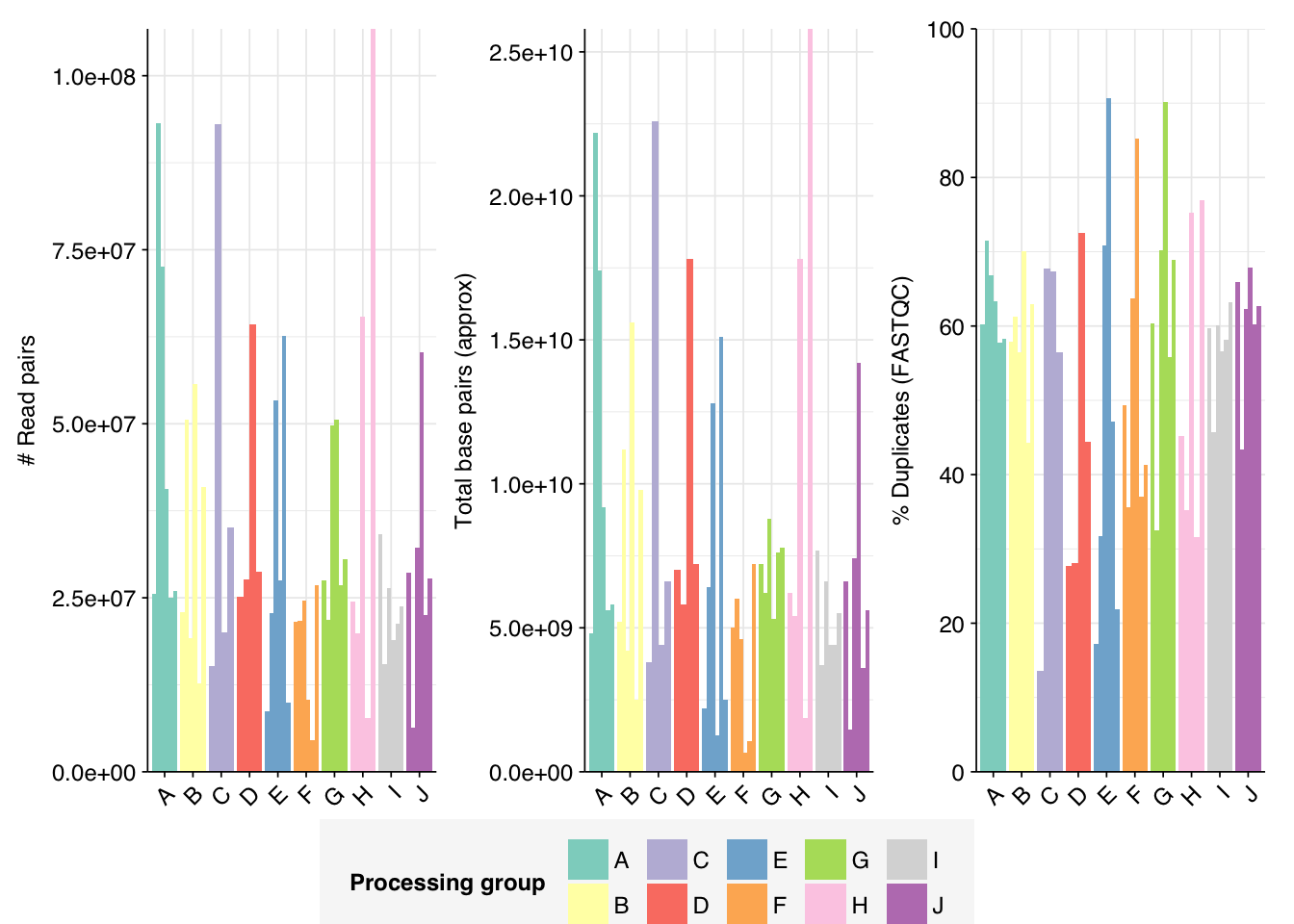
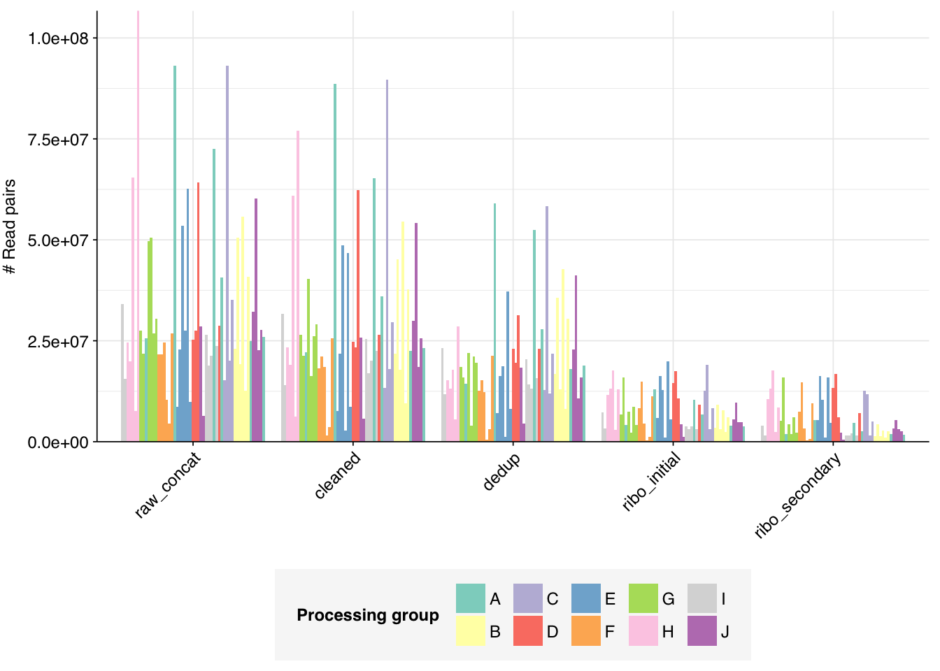
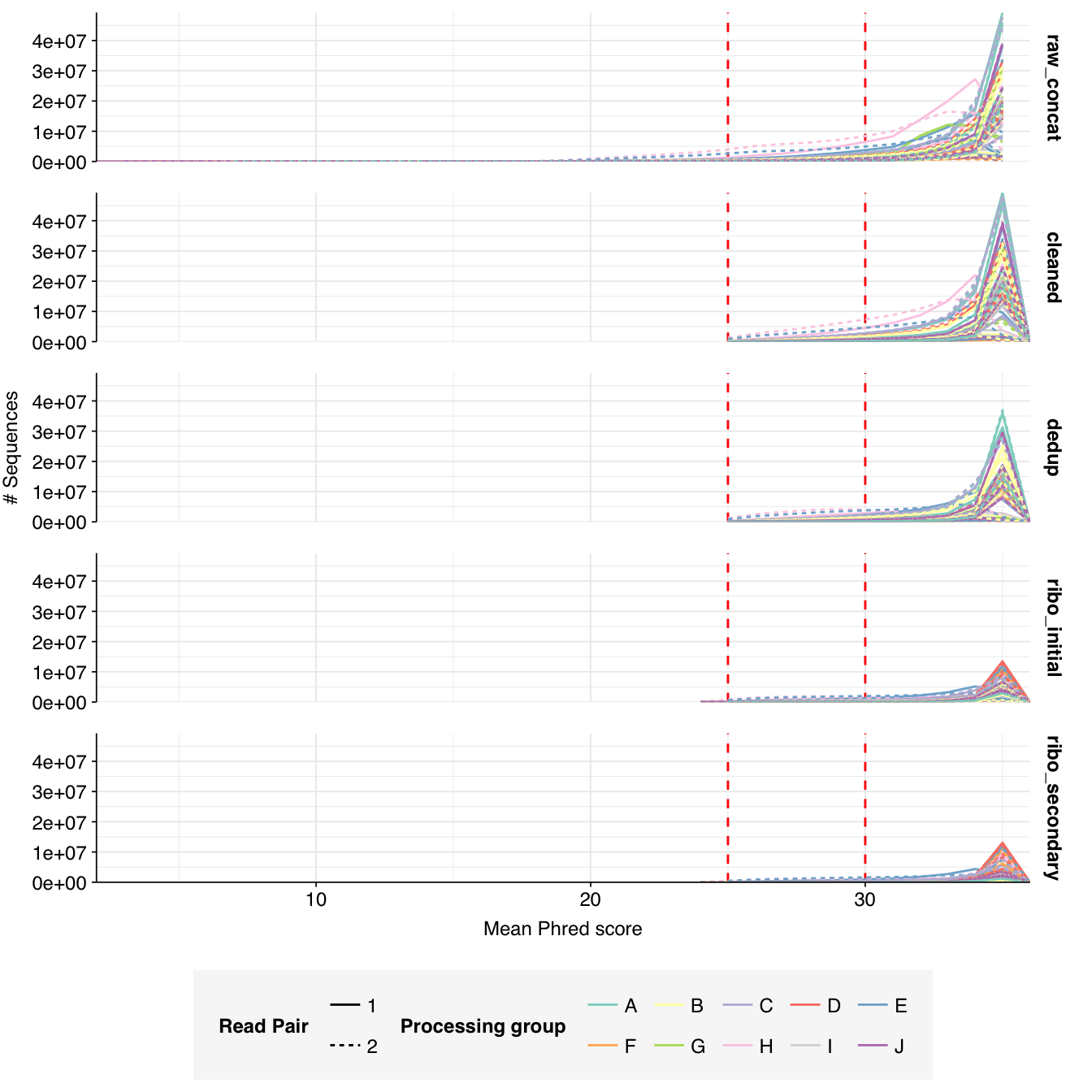
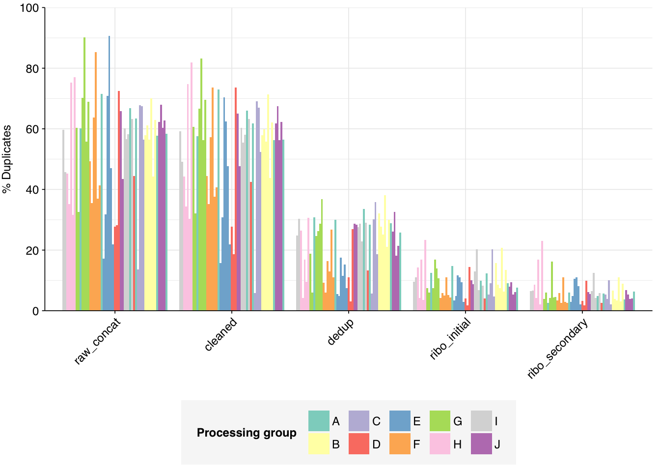
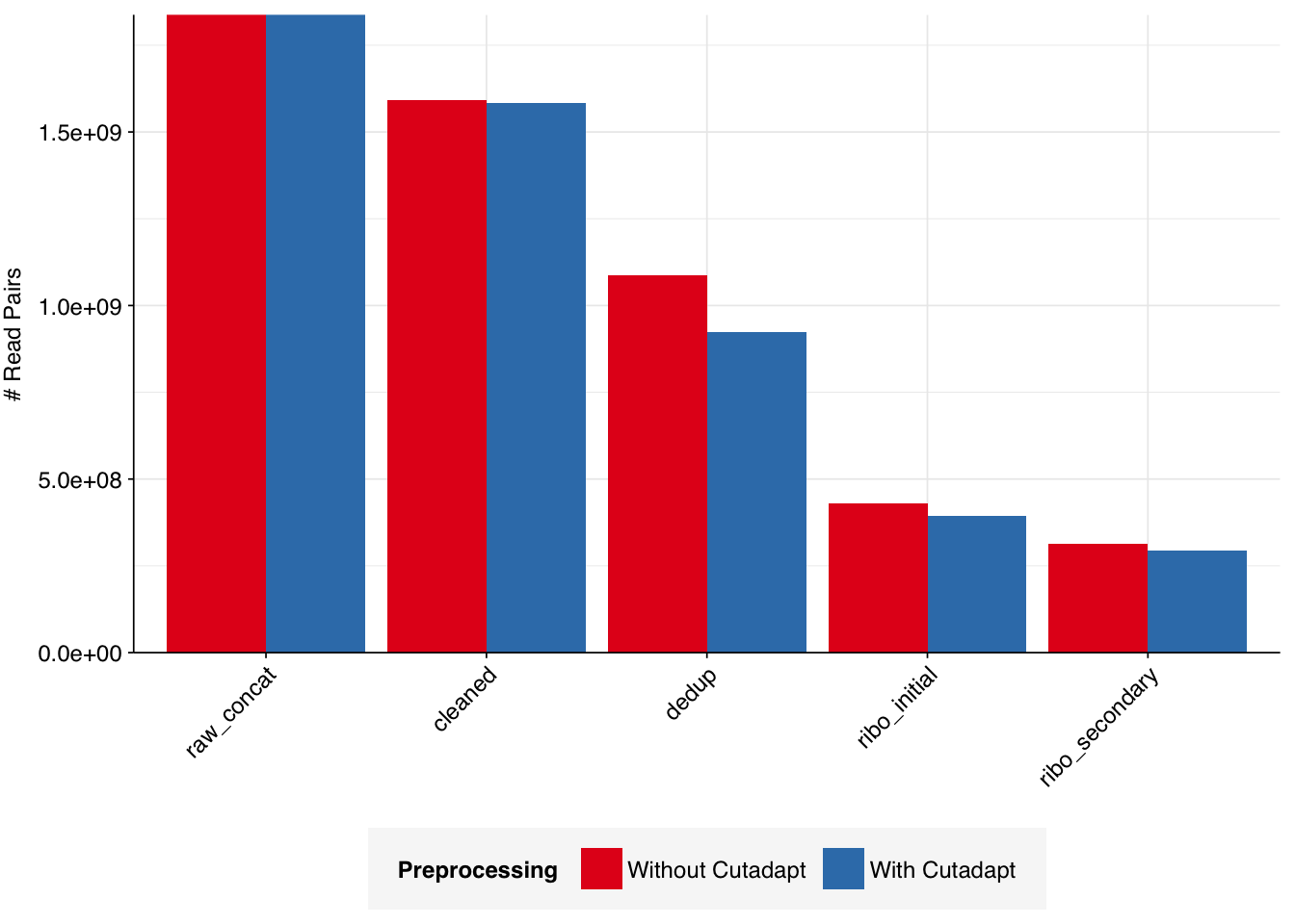
The Spurbeck data comprises 55 samples from 8 processing groups, with 4 to 6 samples per group. The number of sequencing read pairs per sample varied widely from 4.5M-106.7M (mean 33.4M). Taken together, the samples totaled roughly 1.8B read pairs (425 gigabases of sequence). Read qualities were generally high but in need of some light preprocessing. Adapter levels were moderate. Inferred duplication levels were fairly high: 14-91% with a mean of 55%.
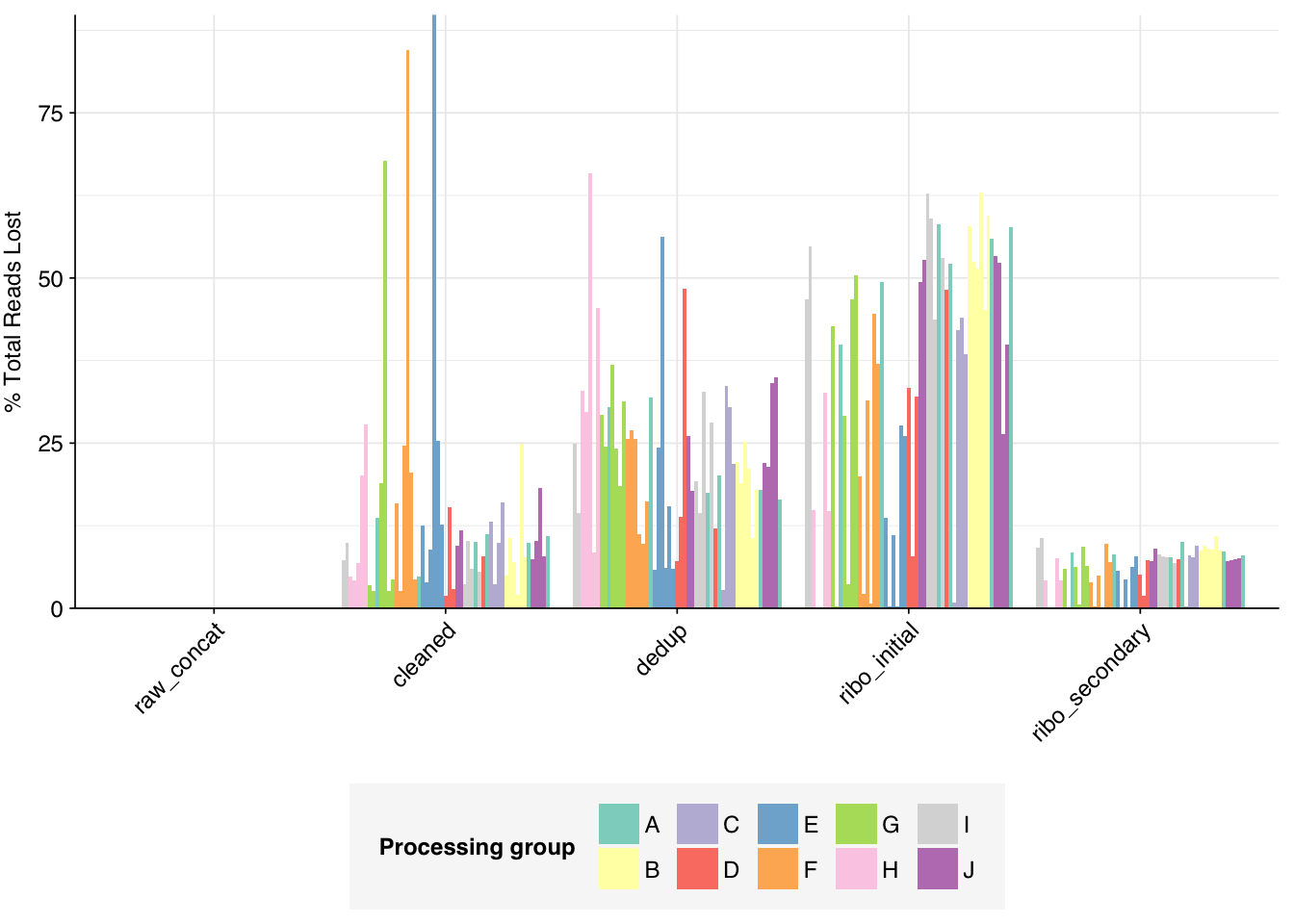
The average fraction of reads lost at each stage in the preprocessing pipeline is shown in the following table. Significant numbers of reads were lost at each stage in the preprocessing pipeline. In total, cleaning, deduplication and initial ribodepletion removed 17-96% (mean 72%) of input reads, while secondary ribodepletion removed an additional 0-11% (mean 6%).
# Plot reads over preprocessingg_reads_stages<-ggplot(basic_stats, aes(x=stage, y=n_read_pairs,fill=group,group=sample))+geom_col(position="dodge")+scale_fill_grp()+scale_y_continuous("# Read pairs", expand=c(0,0))+theme_kitg_reads_stages
Code
# Plot relative read losses during preprocessingg_reads_rel<-ggplot(n_reads_rel, aes(x=stage, y=p_reads_lost_abs_marginal,fill=group,group=sample))+geom_col(position="dodge")+scale_fill_grp()+scale_y_continuous("% Total Reads Lost", expand=c(0,0), labels =function(x)x*100)+theme_kitg_reads_rel
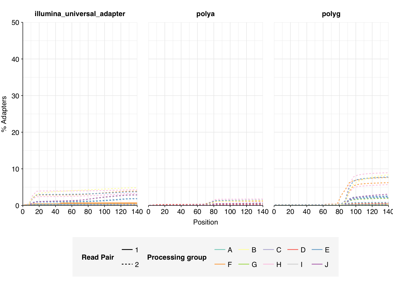
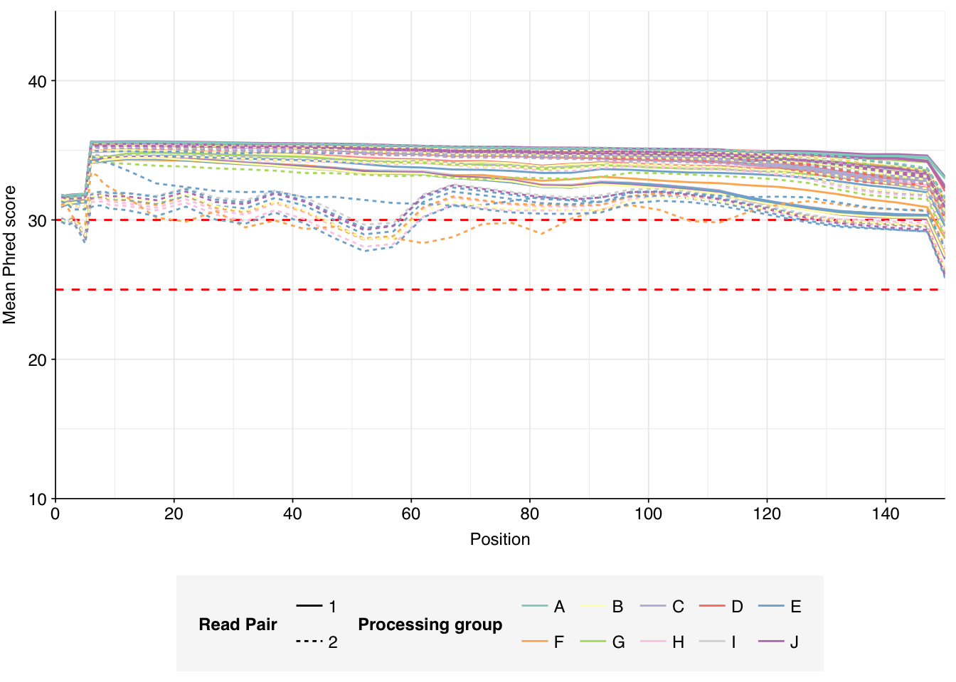
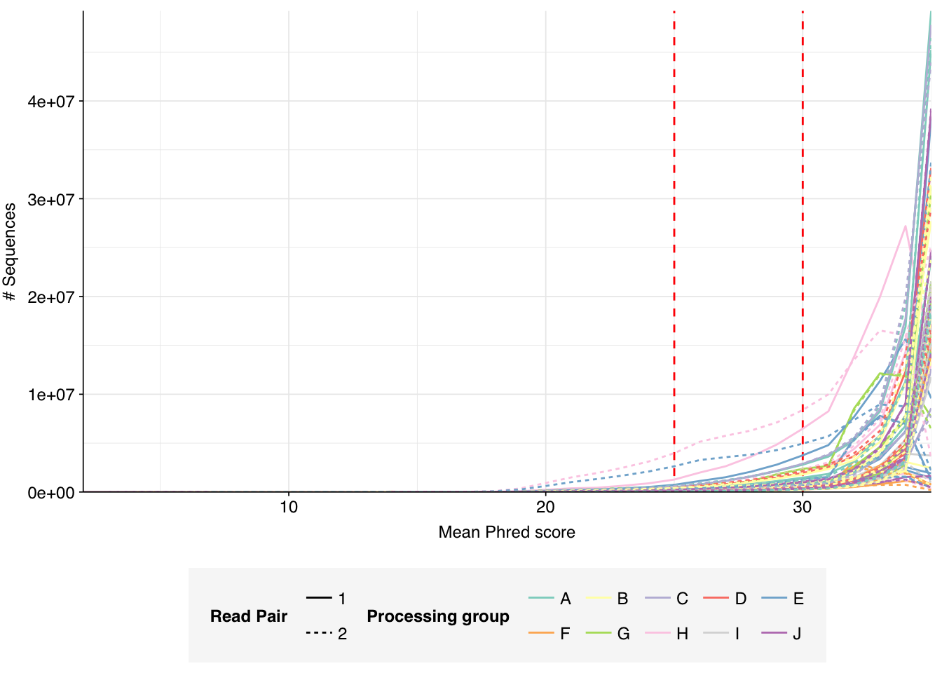
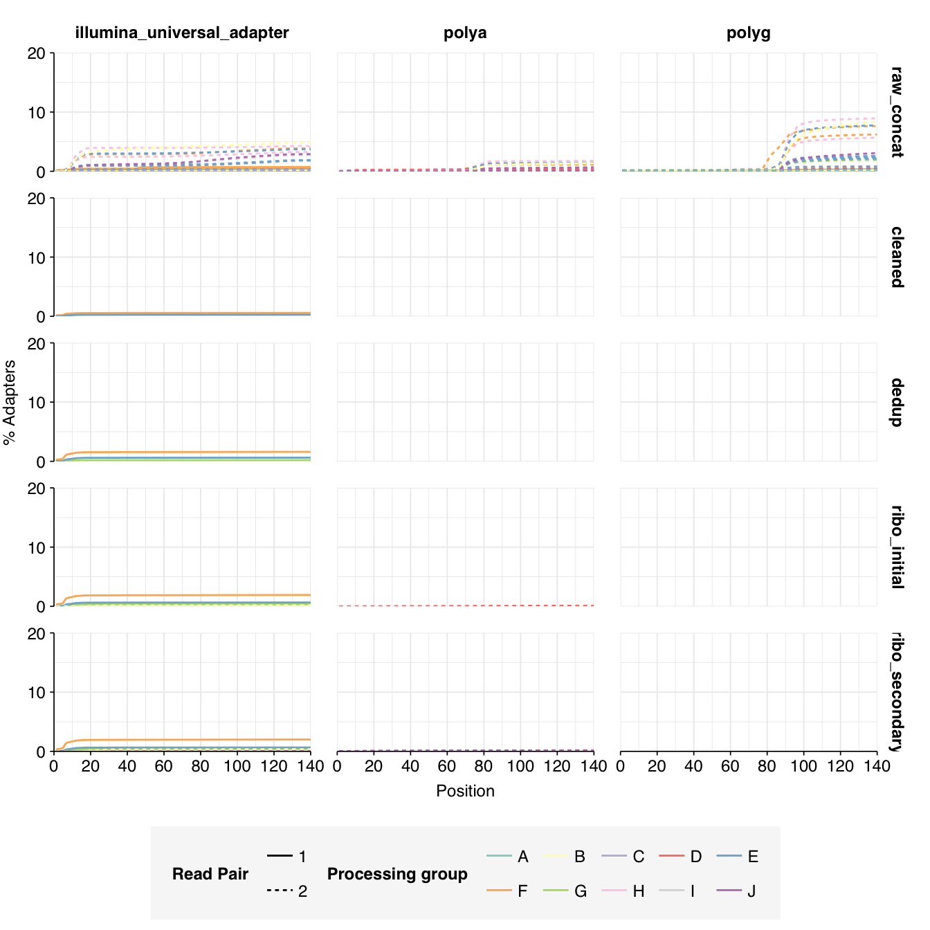
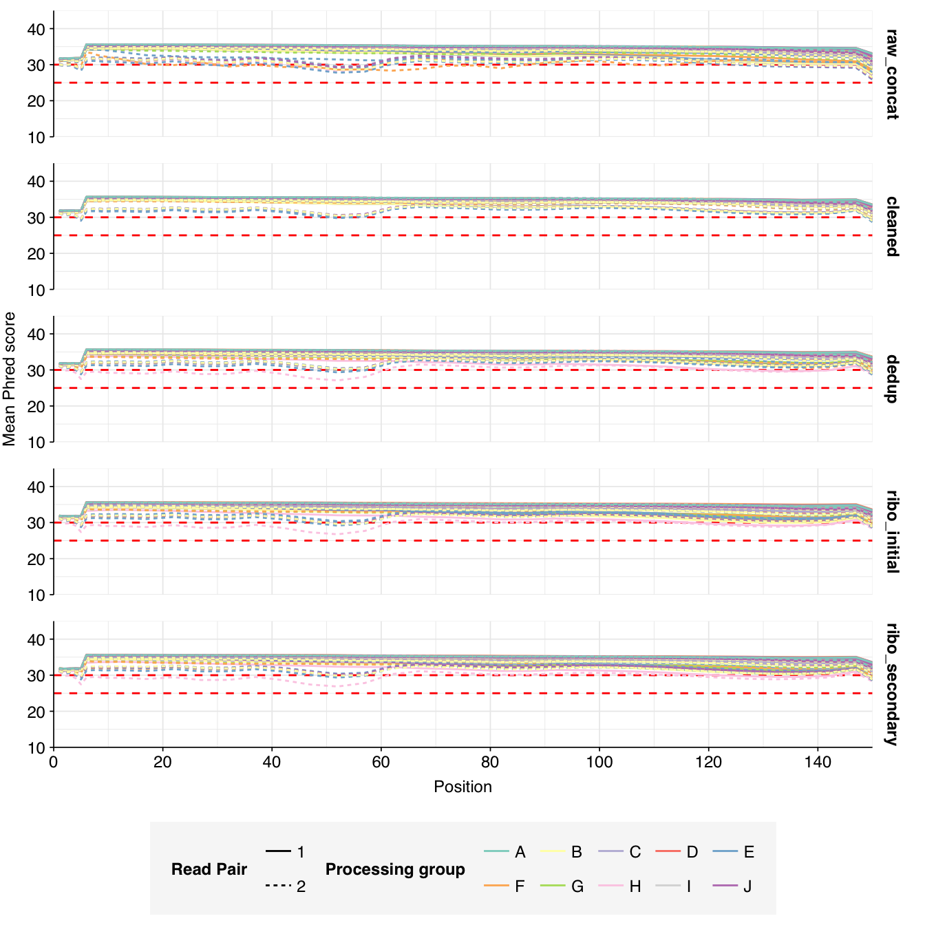
Data cleaning with FASTP was mostly successful at removing adapters; however, detectable levels of Illumina Universal Adapter sequences persisted through the preprocessing pipeline. FASTP was successful at improving read quality.
According to FASTQC, deduplication was quite effective at reducing measured duplicate levels, with FASTQC-measured levels falling from an average of 55% to one of 22%:
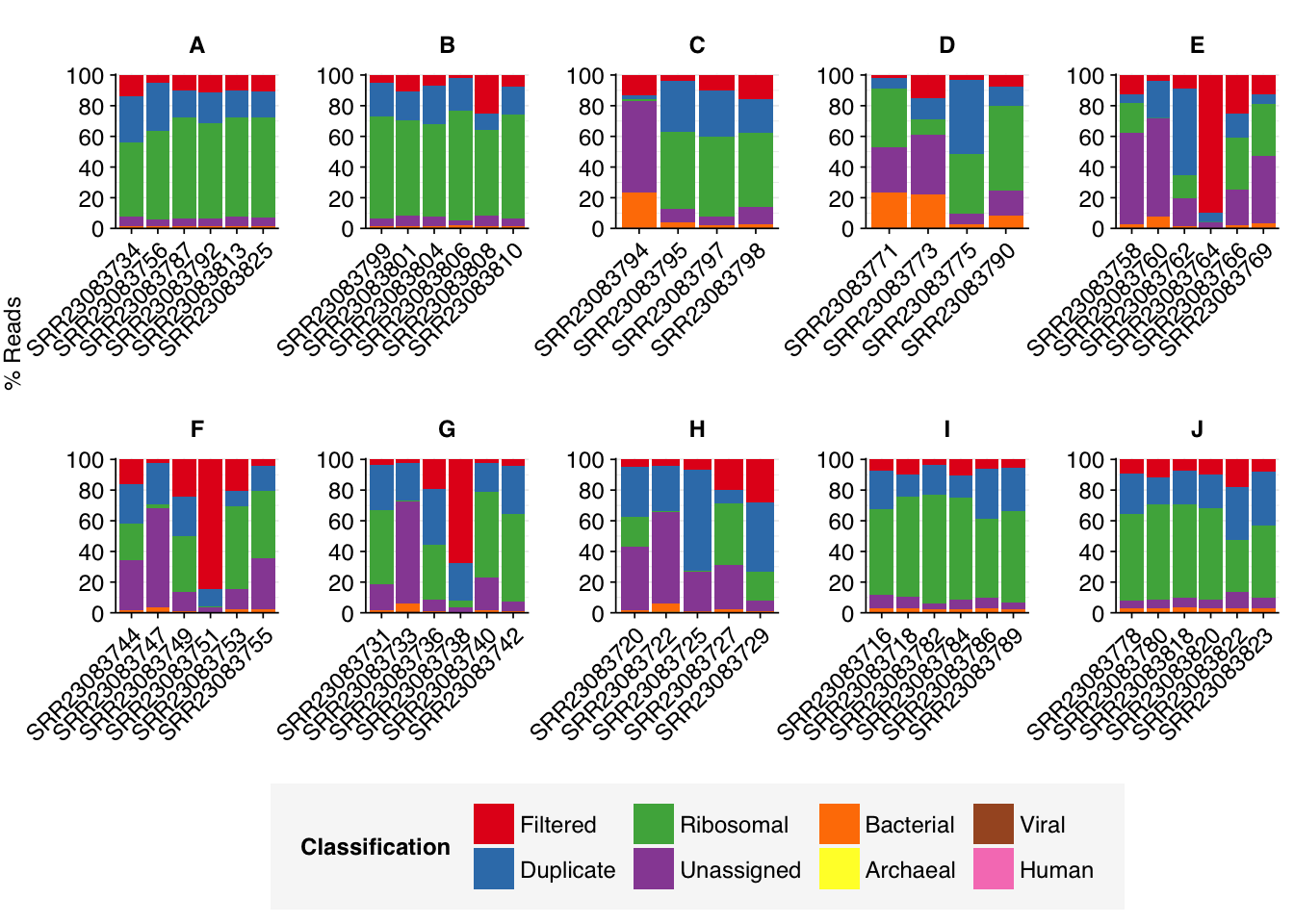
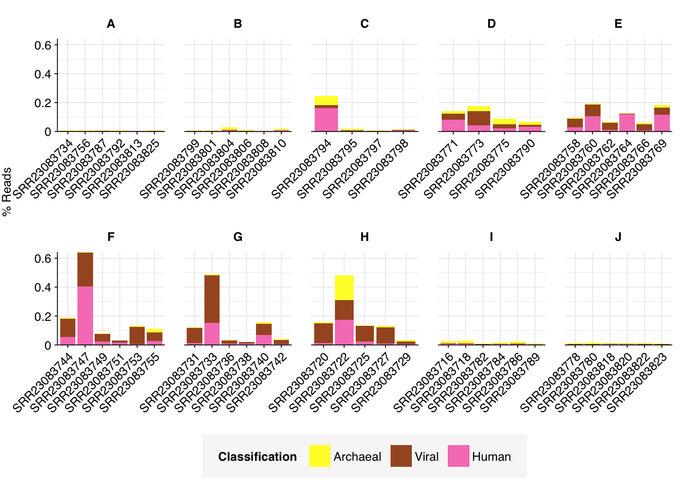
As before, to assess the high-level composition of the reads, I ran the ribodepleted files through Kraken (using the Standard 16 database) and summarized the results with Bracken. Combining these results with the read counts above gives us a breakdown of the inferred composition of the samples:
Average composition varied substantially between groups. Four groups (A, B, I, J) showed high within-group consistency, with high levels of ribosomal reads and very low levels of assigned reads. Other groups showed much more variability between samples, with higher average levels of assigned reads.
Overall, the average relative abundance of viral reads was 0.04%; however, groups F, G & H showed substantially higher average abundance of around 0.1%. Even these elevated groups, however, still show lower total viral abundance than Rothman or Crits-Christoph, so this doesn’t seem particularly noteworthy.
Human-infecting virus reads: validation, round 1
Next, I investigated the human-infecting virus read content of these unenriched samples, using a pipeline identical to that described in my entry on unenriched Rothman samples. This process identified a total of 31,610 read pairs across all samples (0.007% of surviving reads):
To analyze all these reads in a reasonable amount of time, I set up a dedicated EC2 instance, downloaded nt, and ran BLASTN locally there, otherwise using the same parameters I’ve used for past datasets:
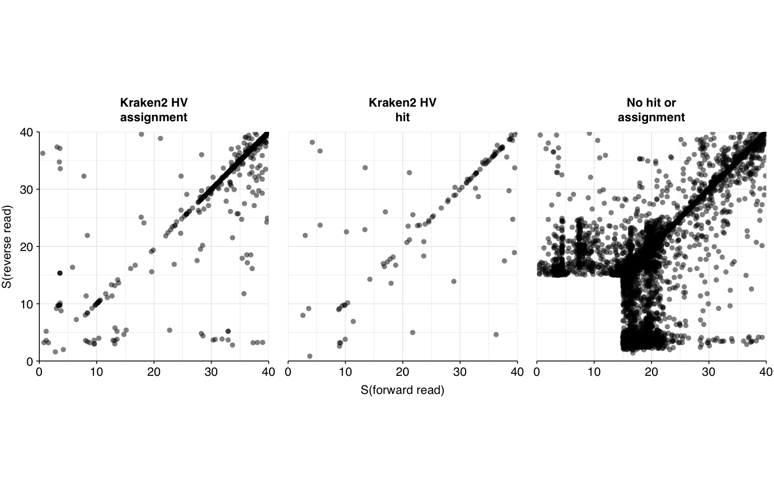
There results were…okay. There were a lot of false positives, but nearly all of them were low-scoring and excluded by my usual score filters. Most true positives, meanwhile, had high enough scores to be retained by those filters. However, there were enough high-scoring false positives and low-scoring true positives to drag down my precision and sensitivity, resulting in an F1 score (at a disjunctive score threshold of 20) a little under 90% – quite a few percentage points lower than I usually aim for.
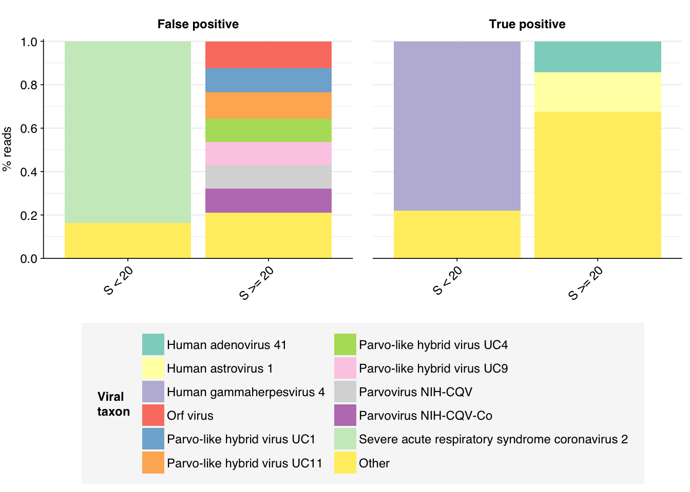
Digging into taxonomic assignments more deeply, we find that low-scoring false positives are primarily mapped by Bowtie2 to SARS-CoV-2, while higher-scoring false positives are mainly mapped to a variety of parvoviruses and parvo-like viruses, as well as Orf virus (cows again?). High-scoring true positives map to a wide range of viruses, but low-scoring true-positives primarily map to human gammaherpesvirus 4. Given that the latter is a DNA virus, I find this quite suspicious.
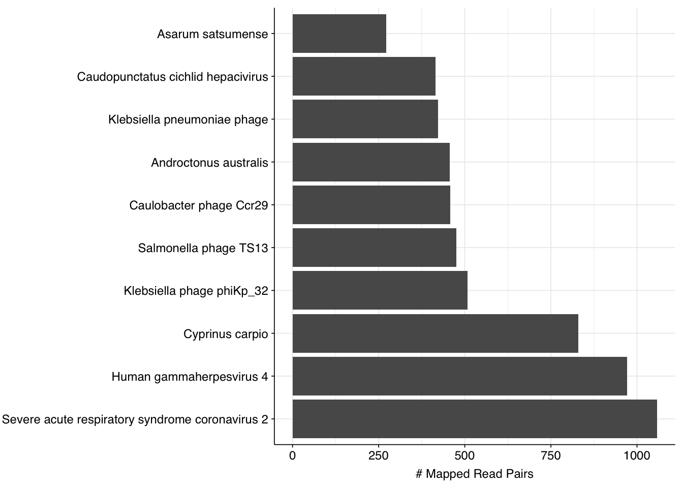
Since sensitivity is more of a problem here than precision, I decided to dig into into the “true positive” herpesvirus reads. There are 1,197 of these in total, 93% of which are low scoring. When I look into the top taxids that BLAST maps these reads to, we see the following:
Two things strike me as notable about these results. First, human gammaherpesvirus 4 is only the second-most-common subject taxid, after SARS-CoV-2, an unrelated virus with a different nucleic-acid type. Hmm. Second, close behind these two viruses is a distinctly non-viral taxon, the common carp. This jumped out at me, because the common carp genome is somewhat notorious for being contaminated with Illumina adapter sequences. This makes me suspect that Illumina adapter contamination is playing a role in these results.
Inspecting these reads manually, I find that a large fraction do indeed show substantial adapter content. In particular, of the 1658 individual reads queried, at least 1338 (81%) showed a strong match to the Illumina multiplexing primer. As such, better removal of these adapter sequences would likely remove most or all of these “false true positives”, potentially significantly improving my results for this dataset.
Human-infecting virus reads: validation, round 2
To address this problem, I added Cutadapt to the pipeline, using settings that allowed it to trim known adaptors internal to the read:
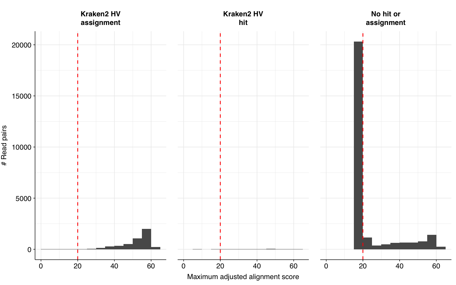
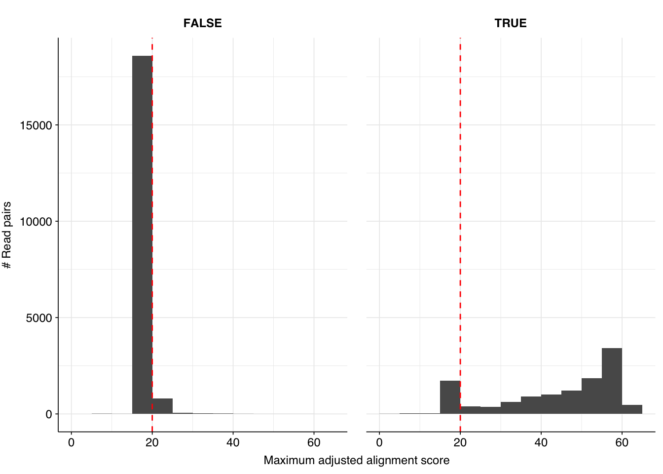
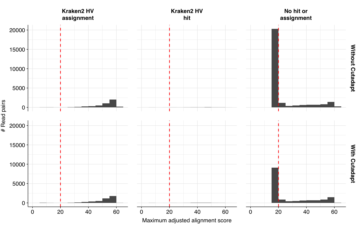
Running this additional preprocessing step reduced the total number of reads surviving cleaning by 10.4M, or an average of 189k reads per sample. The number of putative human-viral reads, meanwhile, was reduced from 31,610 to 19,799, a 37% decrease. This reduction is primarily due to a large decrease in the number of low-scoring Bowtie2-only putative HV hits.
# Make new labelled HV datasetmrg_2<-hv_reads_filtered_2%>%mutate(kraken_label =ifelse(assigned_hv, "Kraken2 HV\nassignment",ifelse(hit_hv, "Kraken2 HV\nhit","No hit or\nassignment")))%>%group_by(sample)%>%arrange(desc(adj_score_fwd), desc(adj_score_rev))%>%mutate(seq_num =row_number(), adj_score_max =pmax(adj_score_fwd, adj_score_rev, na.rm =TRUE))# Merge and plot histogrammrg_2_join<-bind_rows(mrg_1%>%mutate(label="Without Cutadapt"),mrg_2%>%mutate(label="With Cutadapt"))%>%mutate(label =fct_inorder(label))g_hist_2<-ggplot(mrg_2_join, aes(x=adj_score_max))+geom_histogram(binwidth=5,boundary=0,position="dodge")+facet_grid(label~kraken_label)+scale_x_continuous(name ="Maximum adjusted alignment score")+scale_y_continuous(name="# Read pairs")+scale_fill_brewer(palette ="Dark2")+theme_base+geom_vline(xintercept=20, linetype="dashed", color="red")g_hist_2
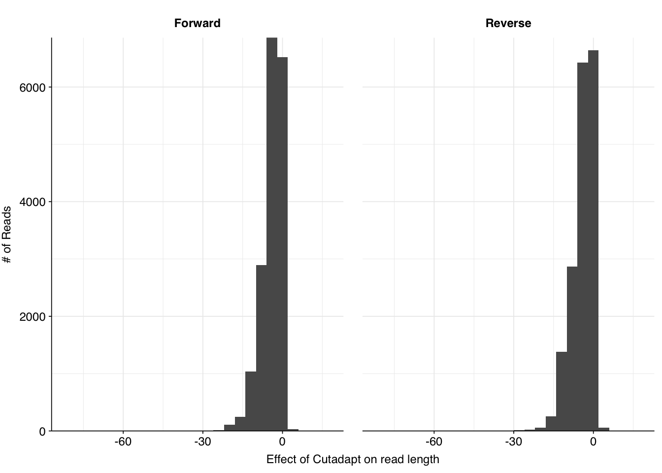
Comparing the lengths of the same sequences in the old versus new results, we see that many reads are reduced in length as a result of adding Cutadapt. As such, it made sense to repeat the BLAST analysis on the reprocessed reads rather than using the BLAST assignments from the previous analysis.
# Import BLAST results (again, pre-filtered to save space)blast_results_2_path<-file.path(data_dir, "putative-viral-blast-best-2.tsv.gz")blast_results_2<-read_tsv(blast_results_2_path, show_col_types =FALSE, col_types =cols(.default="c"))# Filter for best hit for each query/subjectblast_results_2_best<-blast_results_2%>%group_by(qseqid, staxid)%>%filter(bitscore==max(bitscore))%>%filter(length==max(length))%>%filter(row_number()==1)# Rank hits for each queryblast_results_2_ranked<-blast_results_2_best%>%group_by(qseqid)%>%mutate(rank =dense_rank(desc(bitscore)))blast_results_2_highrank<-blast_results_2_ranked%>%filter(rank<=5)%>%mutate(read_pair =str_split(qseqid, "_")%>%sapply(nth, n=-1), seq_num =str_split(qseqid, "_")%>%sapply(nth, n=-2), sample =str_split(qseqid, "_")%>%lapply(head, n=-2)%>%sapply(paste, collapse="_"))%>%mutate(bitscore =as.numeric(bitscore), seq_num =as.numeric(seq_num))# Summarize by read pair and taxidblast_results_2_paired<-blast_results_2_highrank%>%group_by(sample, seq_num, staxid)%>%summarize(bitscore_max =max(bitscore), bitscore_min =min(bitscore), best_rank =min(rank), n_reads =n(), .groups ="drop")# Add viral statusblast_results_2_viral<-blast_results_2_paired%>%mutate(viral =staxid%in%viral_taxa$taxid, viral_full =viral&n_reads==2)# Compare to Kraken & Bowtie assignmentsmrg_2_assign<-mrg_2_num%>%select(sample, seq_num, taxid, assigned_taxid)blast_results_2_assign<-full_join(blast_results_2_viral, mrg_2_assign, by=c("sample", "seq_num"))%>%mutate(taxid_match_bowtie =(staxid==taxid), taxid_match_kraken =(staxid==assigned_taxid), taxid_match_any =taxid_match_bowtie|taxid_match_kraken)blast_results_2_out<-blast_results_2_assign%>%group_by(sample, seq_num)%>%summarize(viral_status =ifelse(any(viral_full), 2,ifelse(any(taxid_match_any), 2,ifelse(any(viral), 1, 0))), .groups ="drop")%>%mutate(viral_status =replace_na(viral_status, 0))
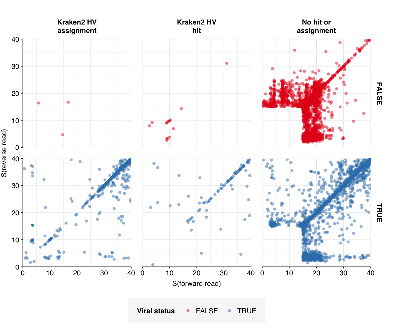
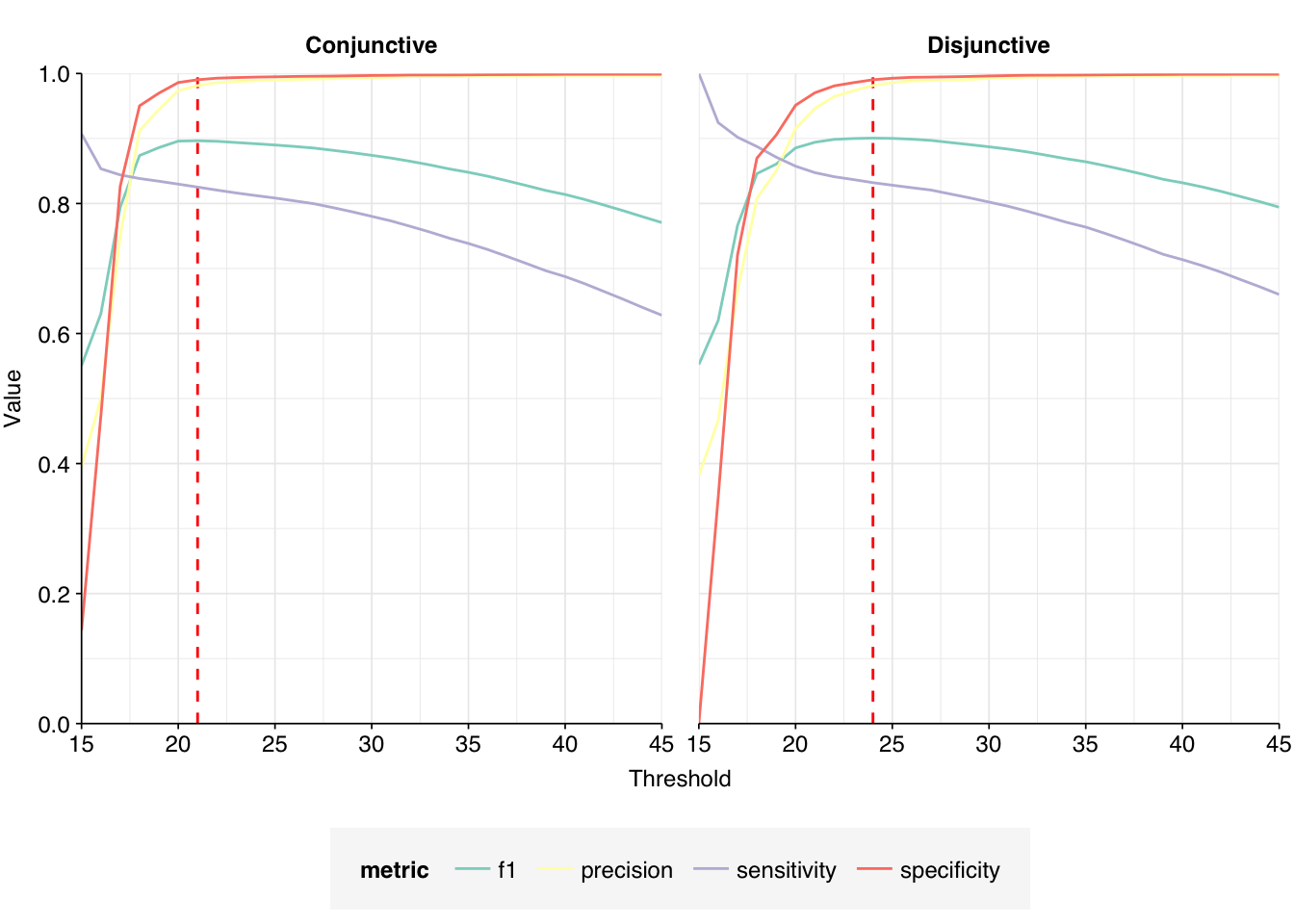
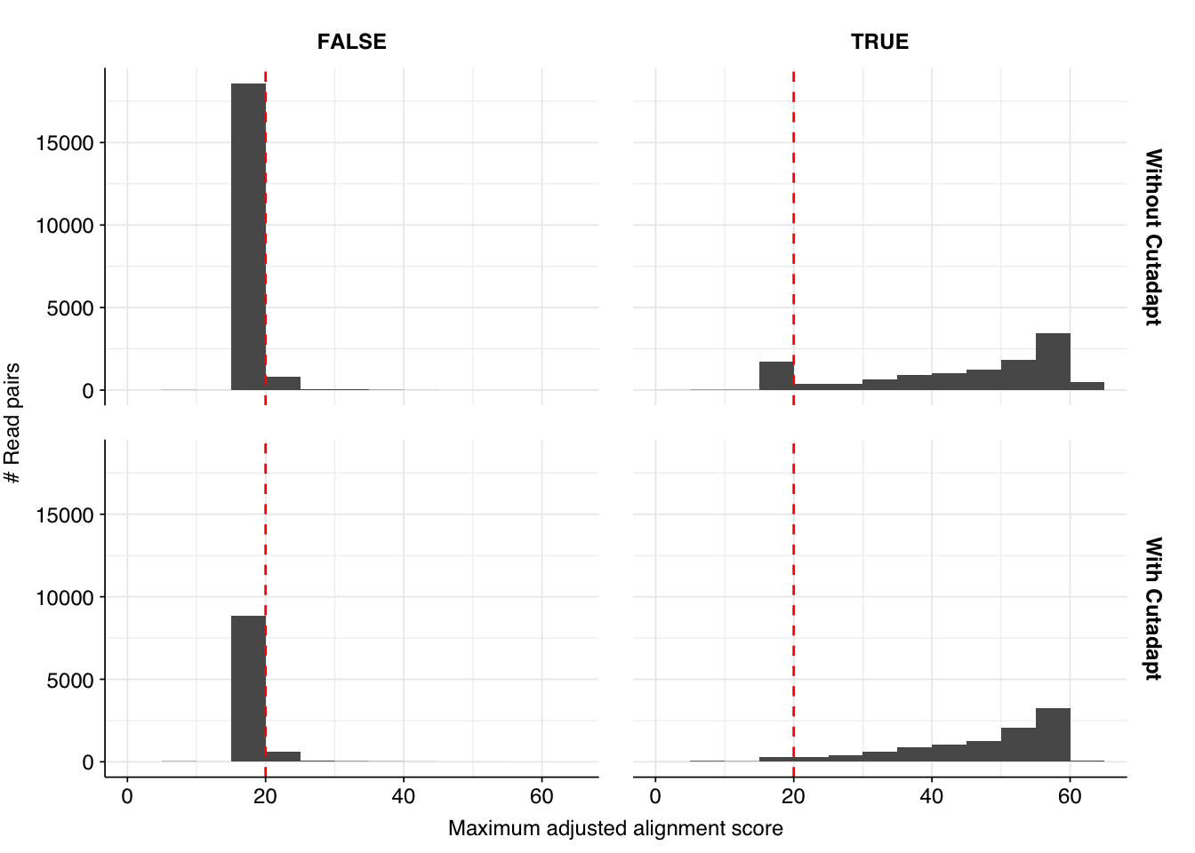
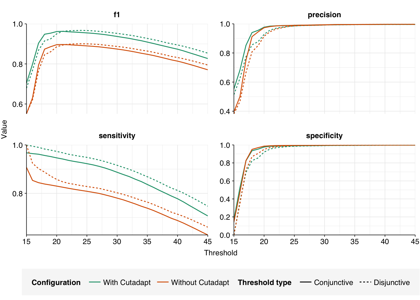
The addition of Cutadapt results in a substantial decrease in low-scoring putative HV sequences, resulting in a large improvement in measured sensitivity and F1 score:
At a disjunctive threshold of 20, excluding “fake true positives” arising from adapter contamination improved measured sensitivity from 86% to 97%, bringing the measured F1 score up from 89% to 95%. I would feel much better about using these results for further downstream analyses.
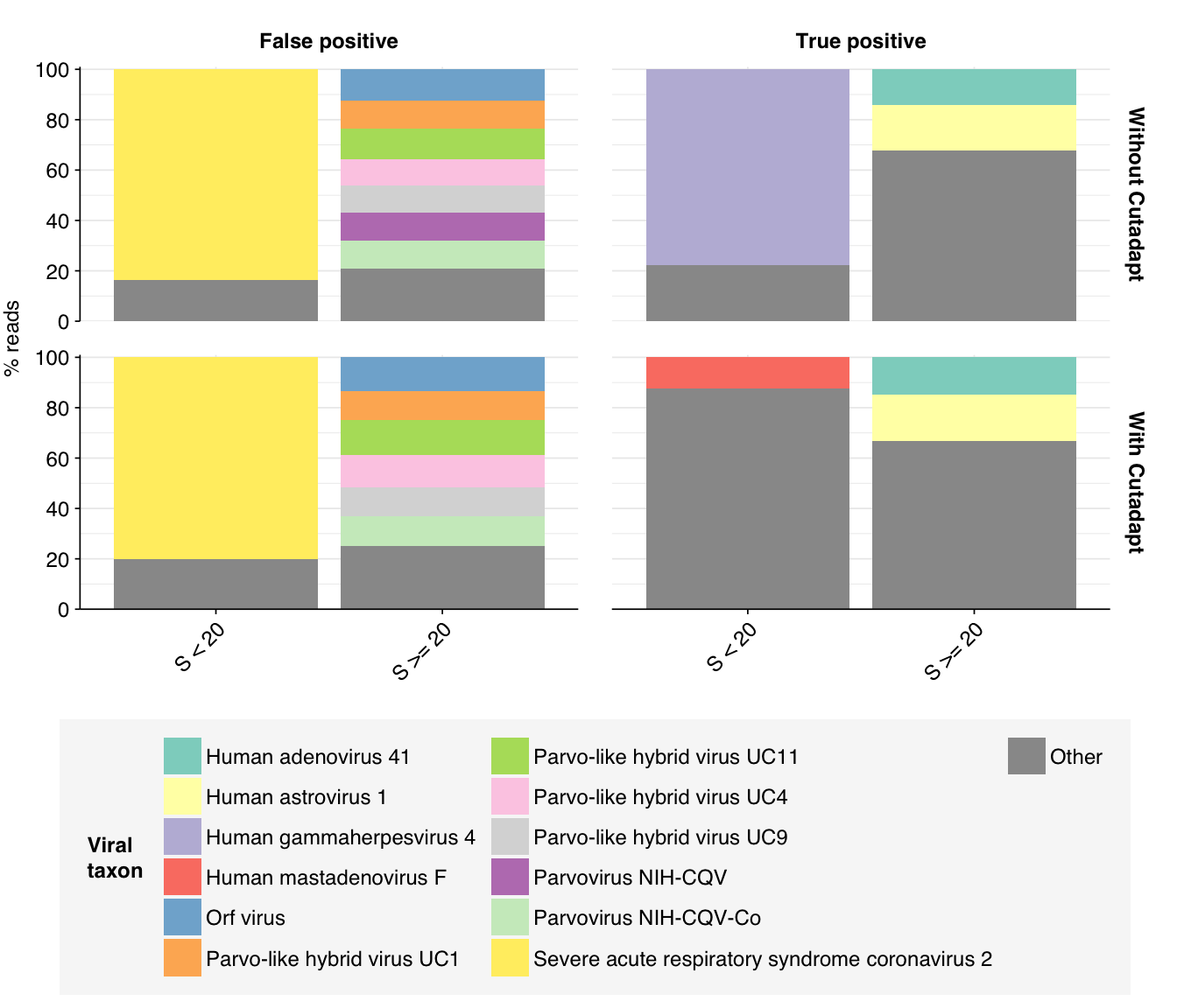
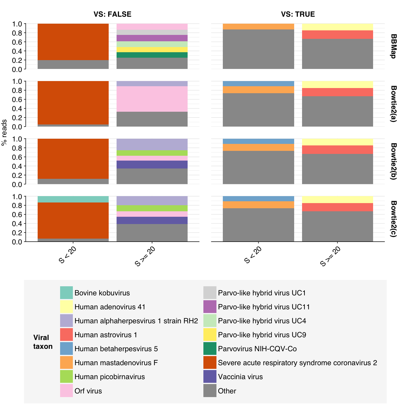
That said, I think further improvement is possible. While addition of Cutadapt processing substantially improved measured sensitivity, measured precision only improved slightly. Looking at the apparent taxonomic makeup of putative HV reads, we see that, while low-scoring “true positives” mapping to herpesviruses have been mostly eliminated, high-scoring false positives still map primarily to parvoviruses and parvo-like viruses:
Not only are these parvoviruses and parvo-like viruses DNA viruses (and thus suspicious as abundant components of the RNA virome), they are also the subject of a famous controversy in early viral metagenomics, where viruses apparently widespread in Chinese hepatitis patients were found to arise from spin column contamination. In fact, these viruses seem not to be human-infecting at all; the authors of the study reporting the contamination suggested that they might be viruses of the diatom algae used as the source of silica for these columns. As such, it seems appropriate to remove these from the human-virus database used to identify putative HV reads.
We also see a significant number of false-positive reads mapped to Orf virus. Historically this has been a sign of contamination with bovine sequences, and indeed the top taxa mapped to these reads by BLAST include Bos taurus (cattle), Bos mutus (wild yak), and Cervus elaphus (red deer).
The ideal approach to removing these false positives would be to add the cow genome to the Kraken database we use for validation of Bowtie2 assignments, along with the pig genome and probably some other known contaminants causing issues. This is probably worth doing at some point, but represents a substantial amount of additional work; I’d rather use a simpler alternative right now if one is available. One option that comes to mind is to try replacing the BBMap aligner I’m using to detect and remove contaminants with Bowtie2; in quick experiments, running Bowtie2 (--sensitive) on the putative Orf virus sequences above, using the same dataset of contaminants for the index, successfully removed about two-thirds of them. While this doesn’t guarantee that Bowtie2 would perform as well on the whole population of contaminating cow sequences, it suggests that using Bowtie2 in place of BBMap is worth trying.
As such, I re-ran the HV detection pipeline again, having made two changes: first, removing Parvovirus NIH-CQV and the parvo-like viruses from the HV database used to identify putative HV reads, and secondly, replacing BBMap with Bowtie2 for contaminant removal.
Human-infecting virus reads: validation, round 3
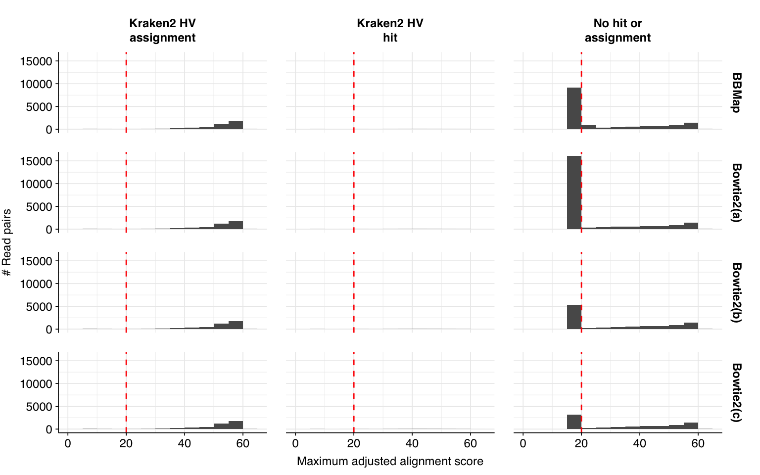
I tried re-running the HV detection pipeline with three different sets of Bowtie2 settings: (a) --sensitive, (b) --local --sensitive-local, and (c) --local --very-sensitive-local. In total, these find 26,370, 15,338 and 13,160 putative human-viral reads, respectively, compared to 31,610 for my initial attempt and 19,799 after the addition of Cutadapt:
# Make new labelled HV datasetmrg_3<-hv_reads_filtered_3%>%mutate(kraken_label =ifelse(assigned_hv, "Kraken2 HV\nassignment",ifelse(hit_hv, "Kraken2 HV\nhit","No hit or\nassignment")))%>%group_by(sample)%>%arrange(desc(adj_score_fwd), desc(adj_score_rev))%>%mutate(seq_num =row_number(), adj_score_max =pmax(adj_score_fwd, adj_score_rev, na.rm =TRUE))# Merge and plot histogrammrg_join_3<-bind_rows(mrg_2%>%mutate(attempt="BBMap"), mrg_3)g_hist_3<-ggplot(mrg_join_3, aes(x=adj_score_max))+geom_histogram(binwidth=5,boundary=0,position="dodge")+facet_grid(attempt~kraken_label)+scale_x_continuous(name ="Maximum adjusted alignment score")+scale_y_continuous(name="# Read pairs")+scale_fill_brewer(palette ="Dark2")+theme_base+geom_vline(xintercept=20, linetype="dashed", color="red")g_hist_3
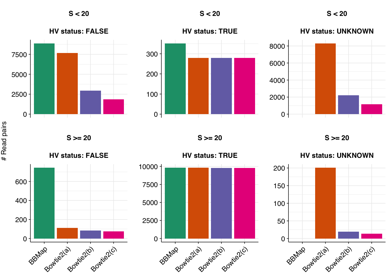
In all cases, the great majority of false-positive sequences from previous attempts were successfully removed (85%/89%/90%, respectively), along with a small number of true-positives (0.19%/0.23%/0.23%, respectively). At the same time, a number of new putative HV sequences arose as a result of the change in filtering algorithm: 8,512/2,224/1,166 respectively. The great majority of these (97.6%/99.1%/98.8%) are low-scoring, suggesting that they are mostly or entirely false matches that are being let through by Bowtie2 that were previously being caught by BBMap.
Warning: The `<scale>` argument of `guides()` cannot be `FALSE`. Use "none" instead as
of ggplot2 3.3.4.
Code
g_status_summ
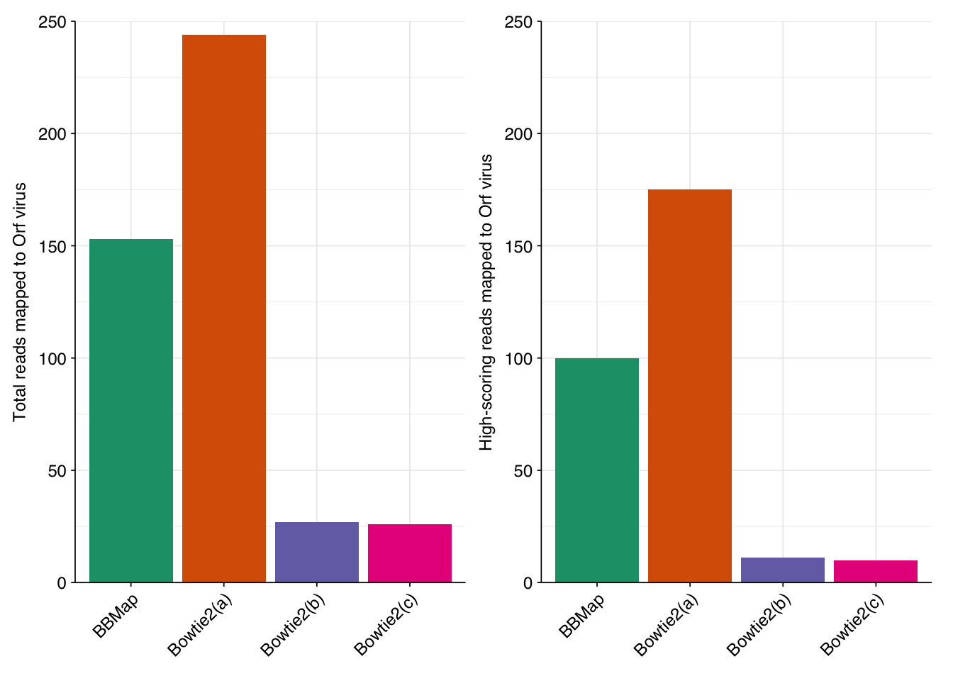
Checking putative Orf virus reads specifically, all three Bowtie2-based attempts successfully remove most putative Orf reads from the previous attempt, while introducing some number of new putative hits (of which I assume the vast majority are fake hits arising from bovine contamination). In attempt (a), these new putative hits outnumber the old hits that were removed, resulting in a net increase in putative (but, I’m fairly confident, false) Orf-virus hits, whether total or high-scoring. Conversely, attempts (b) and (c) manage to remove even more old putative Orf hits while creating many fewer new ones, resulting in a large net decrease in total and high-scoring putative Orf hits:
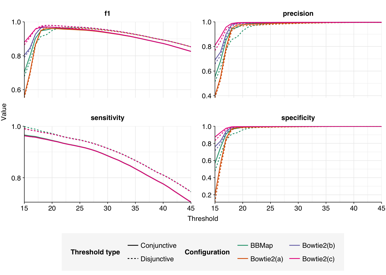
Next, I validated all new putative HV sequences with BLASTN as before, then evaluated each attempt’s performance against all the putative HV reads identified by any attempt:
At a disjunctive threshold of 20, Bowtie2(c) (--very-sensitive-local) performs the best, with an F1 score of 0.979; Bowtie2(b) (--sensitive-local) is very close behind. In both cases, precision (>=0.988) is higher than sensitivity (~0.969), suggesting that any further improvements would come from investigating low-scoring true-positives:
I suspect that small additional gains are possible here, since I’m suspicious about the low-scoring “true-positives” mapping to human betaherpesvirus 5 and human mastadenovirus F. However, I’ve already spent a long time optimizing the results for this dataset, and the results are now good enough that I feel okay with leaving this here. Going forward, I’ll use Bowtie2(c) as my alignment strategy for the HV identification pipeline.
Human-infecting virus reads: analysis
After several rounds of validation and refinement, we finally come to actually analyzing the human-infecting virus content of Spurbeck et al. This section might seem disappointingly short compared to all the effort expended to get here.
Code
# Get raw read countsread_counts_raw<-basic_stats_raw%>%select(sample, group, date, n_reads_raw =n_read_pairs)# Get HV read counts & RAmrg_hv<-mrg_3%>%filter(attempt=="Bowtie2(c)")%>%mutate(hv_status =assigned_hv|hit_hv|adj_score_max>=20)read_counts_hv<-mrg_hv%>%filter(hv_status)%>%group_by(sample)%>%count(name ="n_reads_hv")read_counts<-read_counts_raw%>%left_join(read_counts_hv, by="sample")%>%mutate(n_reads_hv =replace_na(n_reads_hv, 0), p_reads_hv =n_reads_hv/n_reads_raw)# Aggregateread_counts_group<-read_counts%>%group_by(group)%>%summarize(n_reads_raw =sum(n_reads_raw), n_reads_hv =sum(n_reads_hv))%>%mutate(p_reads_hv =n_reads_hv/n_reads_raw)read_counts_total<-read_counts_group%>%ungroup%>%summarize(n_reads_raw =sum(n_reads_raw), n_reads_hv =sum(n_reads_hv))%>%mutate(p_reads_hv =n_reads_hv/n_reads_raw, group ="All groups")read_counts_agg<-read_counts_group%>%bind_rows(read_counts_total)%>%arrange(group)%>%arrange(str_detect(group, "All groups"))%>%mutate(group =fct_inorder(group))
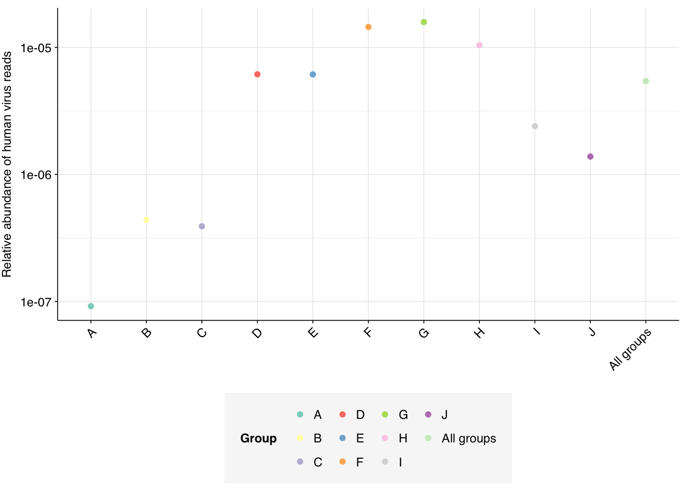
Applying a disjunctive cutoff at S=20 identifies 9,990 reads as human-viral out of 1.84B total reads, for a relative HV abundance of \(5.44 \times 10^{-6}\). This compares to \(2.8 \times 10^{-4}\) on the public dashboard, corresponding to the results for Kraken-only identification: a roughly 2x increase, smaller than the 4-5x increases seen for Crits-Christoph and Rothman. Relative HV abundances for individual sample groups ranged from \(9.19 \times 10^{-8}\) to \(1.58 \times 10^{-5}\); as with total virus reads, groups F, G & H showed the highest relative abundance:
Code
# Visualizeg_phv_agg<-ggplot(read_counts_agg, aes(x=group, y=p_reads_hv, color=group))+geom_point()+scale_y_log10("Relative abundance of human virus reads")+scale_color_brewer(palette ="Set3", name ="Group")+theme_kitg_phv_agg
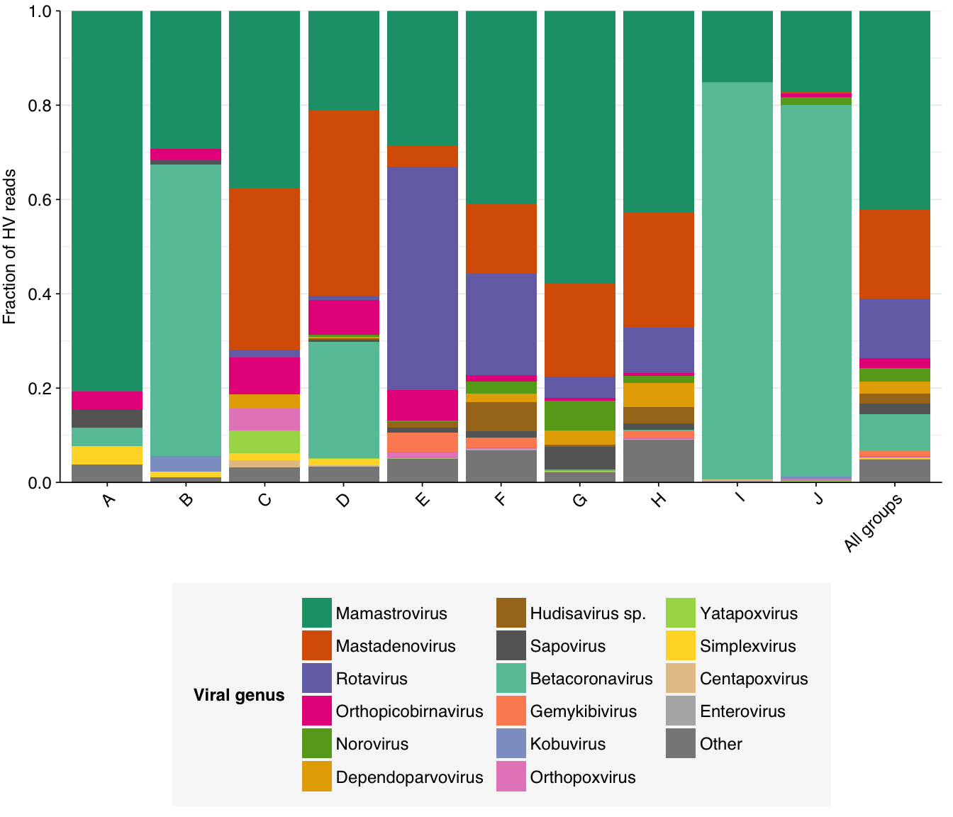
Digging into particular viruses, we see that Mamastrovirus, Mastadenovirus, Rotavirus and Betacoronavirus are the most abundant genera across samples:
Code
# Get viral taxon names for putative HV readsviral_taxa$name[viral_taxa$taxid==249588]<-"Mamastrovirus"viral_taxa$name[viral_taxa$taxid==194960]<-"Kobuvirus"viral_taxa$name[viral_taxa$taxid==688449]<-"Salivirus"viral_taxa$name[viral_taxa$taxid==694002]<-"Betacoronavirus"viral_taxa$name[viral_taxa$taxid==694009]<-"SARS-CoV"viral_taxa$name[viral_taxa$taxid==694003]<-"Betacoronavirus 1"viral_taxa$name[viral_taxa$taxid==568715]<-"Astrovirus MLB1"viral_taxa$name[viral_taxa$taxid==194965]<-"Aichivirus B"mrg_hv_named<-mrg_hv%>%left_join(viral_taxa, by="taxid")# Discover viral species & genera for HV readsraise_rank<-function(read_db, taxid_db, out_rank="species", verbose=FALSE){# Get higher ranks than search rankranks<-c("subspecies", "species", "subgenus", "genus", "subfamily", "family", "suborder", "order", "class", "subphylum", "phylum", "kingdom", "superkingdom")rank_match<-which.max(ranks==out_rank)high_ranks<-ranks[rank_match:length(ranks)]# Merge read DB and taxid DBreads<-read_db%>%select(-parent_taxid, -rank, -name)%>%left_join(taxid_db, by="taxid")# Extract sequences that are already at appropriate rankreads_rank<-filter(reads, rank==out_rank)# Drop sequences at a higher rank and return unclassified sequencesreads_norank<-reads%>%filter(rank!=out_rank, !rank%in%high_ranks, !is.na(taxid))while(nrow(reads_norank)>0){# As long as there are unclassified sequences...# Promote read taxids and re-merge with taxid DB, then re-classify and filterreads_remaining<-reads_norank%>%mutate(taxid =parent_taxid)%>%select(-parent_taxid, -rank, -name)%>%left_join(taxid_db, by="taxid")reads_rank<-reads_remaining%>%filter(rank==out_rank)%>%bind_rows(reads_rank)reads_norank<-reads_remaining%>%filter(rank!=out_rank, !rank%in%high_ranks, !is.na(taxid))}# Finally, extract and append reads that were excluded during the processreads_dropped<-reads%>%filter(!seq_id%in%reads_rank$seq_id)reads_out<-reads_rank%>%bind_rows(reads_dropped)%>%select(-parent_taxid, -rank, -name)%>%left_join(taxid_db, by="taxid")return(reads_out)}hv_reads_genera<-raise_rank(mrg_hv_named, viral_taxa, "genus")# Count relative abundance for generahv_genera_counts_raw<-hv_reads_genera%>%group_by(group, name)%>%summarize(n_reads_hv =sum(hv_status), .groups ="drop")%>%inner_join(read_counts_agg%>%select(group, n_reads_raw), by="group")hv_genera_counts_all<-hv_genera_counts_raw%>%group_by(name)%>%summarize(n_reads_hv =sum(n_reads_hv), n_reads_raw =sum(n_reads_raw))%>%mutate(group ="All groups")hv_genera_counts_agg<-bind_rows(hv_genera_counts_raw, hv_genera_counts_all)%>%mutate(p_reads_hv =n_reads_hv/n_reads_raw)# Compute ranks for species and genera and restrict to high-ranking taxamax_rank_genera<-5hv_genera_counts_ranked<-hv_genera_counts_agg%>%group_by(group)%>%mutate(rank =rank(desc(n_reads_hv), ties.method="max"), highrank =rank<=max_rank_genera)%>%group_by(name)%>%mutate(highrank_any =any(highrank), name_display =ifelse(highrank_any, name, "Other"))%>%group_by(name_display)%>%mutate(mean_rank =mean(rank))%>%arrange(mean_rank)%>%ungroup%>%mutate(name_display =fct_inorder(name_display))%>%arrange(str_detect(group, "Other"))%>%mutate(group =fct_inorder(group))# Plot compositionpalette_rank<-c(brewer.pal(8, "Dark2"), brewer.pal(8, "Set2"), "#888888")g_vcomp_genera<-ggplot(hv_genera_counts_ranked, aes(x=group, y=n_reads_hv, fill=name_display))+geom_col(position ="fill")+scale_fill_manual(values =palette_rank, name ="Viral genus")+scale_y_continuous(name ="Fraction of HV reads", breaks =seq(0,1,0.2), expand =c(0,0))+guides(fill =guide_legend(ncol=3))+theme_kitg_vcomp_genera
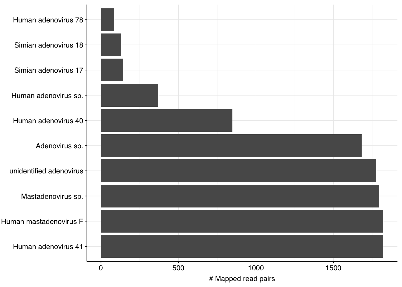
Mamastrovirus and Rotavirus are predominantly enteric RNA viruses whose prominence here makes sense, while the prevalence of Betacoronavirus is probably a result of the ongoing SARS-CoV-2 pandemic. As a DNA virus, the abundance of Mastadenovirus is a bit more surprising; however, this finding is consistent with the public dashboard, and is also borne out by the other BLASTN matches for these sequences, all of which are other adenovirus taxa:
Compared to the last few datasets I analyzed, the analysis of Spurbeck took a long time, numerous attempts, and a lot of computational resources. However, as I said at the start of this post, I’m happy with the outcome and am confident it will improve analysis of future datasets. While the overall prevalence of human-infecting viruses is fairly low in Spurbeck compared to other wastewater datasets I’ve looked at, its inclusion as a core dataset for the P2RA analysis make it especially important to process in a reliable and high-quality manner.
Next, I’ll turn my attention to more datasets included in the P2RA analysis, as well as some air-sampling datasets we’re interested in for another project.
Source Code
---title: "Workflow analysis of Spurbeck et al. (2023)"subtitle: "Cave carpa."author: "Will Bradshaw"date: 2024-04-01format: html: code-fold: true code-tools: true code-link: true df-print: pagededitor: visualtitle-block-banner: black---```{r}#| label: load-packages#| include: falselibrary(tidyverse)library(cowplot)library(patchwork)library(fastqcr)library(RColorBrewer)source("../scripts/aux_plot-theme.R")theme_base <- theme_base +theme(aspect.ratio =NULL)theme_kit <- theme_base +theme(axis.text.x =element_text(hjust =1, angle =45),axis.title.x =element_blank(),)tnl <-theme(legend.position ="none")```Continuing my analysis of datasets from the [P2RA preprint](https://doi.org/10.1101/2023.12.22.23300450), I analyzed the data from Spurbeck et al. (2023), a wastewater RNA-sequencing study from Ohio. Samples for this study underwent a variety of processing protocols at different research centers across the state. Along with Rothman and Crits-Christoph, Spurbeck is one of three RNA-sequencing studies that underwent full in-depth analysis in the P2RA study, so is worth looking at closely here.This one turned out to be a bit of a saga. As we'll see in the section on human-virus identification, it took multiple tries and several substantial changes to the pipeline to get things to a state I was happy with. Still, I am happy with the outcome and think the changes will improve analysis of future datasets.# The raw dataThe Spurbeck data comprises 55 samples from 8 processing groups, with 4 to 6 samples per group. The number of sequencing read pairs per sample varied widely from 4.5M-106.7M (mean 33.4M). Taken together, the samples totaled roughly 1.8B read pairs (425 gigabases of sequence). Read qualities were generally high but in need of some light preprocessing. Adapter levels were moderate. Inferred duplication levels were fairly high: 14-91% with a mean of 55%.```{r}#| warning: false#| label: read-qc-data# Data input pathsdata_dir <-"../data/2024-04-01_spurbeck/"libraries_path <-file.path(data_dir, "sample-metadata.csv")basic_stats_path <-file.path(data_dir, "qc_basic_stats_1.tsv")adapter_stats_path <-file.path(data_dir, "qc_adapter_stats.tsv")quality_base_stats_path <-file.path(data_dir, "qc_quality_base_stats.tsv")quality_seq_stats_path <-file.path(data_dir, "qc_quality_sequence_stats.tsv")# Import libraries and extract metadata from sample nameslibraries <-read_csv(libraries_path, show_col_types =FALSE)# Import QC datastages <-c("raw_concat", "cleaned", "dedup", "ribo_initial", "ribo_secondary")basic_stats <-read_tsv(basic_stats_path, show_col_types =FALSE) %>%# mutate(sample = sub("_2$", "", sample)) %>%inner_join(libraries, by="sample") %>%mutate(stage =factor(stage, levels = stages),sample =fct_inorder(sample))adapter_stats <-read_tsv(adapter_stats_path, show_col_types =FALSE) %>%mutate(sample =sub("_2$", "", sample)) %>%inner_join(libraries, by="sample") %>%mutate(stage =factor(stage, levels = stages),read_pair =fct_inorder(as.character(read_pair)))quality_base_stats <-read_tsv(quality_base_stats_path, show_col_types =FALSE) %>%# mutate(sample = sub("_2$", "", sample)) %>%inner_join(libraries, by="sample") %>%mutate(stage =factor(stage, levels = stages),read_pair =fct_inorder(as.character(read_pair)))quality_seq_stats <-read_tsv(quality_seq_stats_path, show_col_types =FALSE) %>%# mutate(sample = sub("_2$", "", sample)) %>%inner_join(libraries, by="sample") %>%mutate(stage =factor(stage, levels = stages),read_pair =fct_inorder(as.character(read_pair)))# Filter to raw databasic_stats_raw <- basic_stats %>%filter(stage =="raw_concat")adapter_stats_raw <- adapter_stats %>%filter(stage =="raw_concat")quality_base_stats_raw <- quality_base_stats %>%filter(stage =="raw_concat")quality_seq_stats_raw <- quality_seq_stats %>%filter(stage =="raw_concat")``````{r}#| fig-height: 5#| warning: false#| label: plot-basic-stats# Visualize basic statsscale_fill_grp <- purrr::partial(scale_fill_brewer, palette="Set3", name="Processing group")g_basic <-ggplot(basic_stats_raw, aes(x=group, fill=group, group=sample)) +scale_fill_grp() + theme_kitg_nreads_raw <- g_basic +geom_col(aes(y=n_read_pairs), position ="dodge") +scale_y_continuous(name="# Read pairs", expand=c(0,0))g_nreads_raw_2 <- g_nreads_raw +theme(legend.position ="none")legend_group <-get_legend(g_nreads_raw)g_nbases_raw <- g_basic +geom_col(aes(y=n_bases_approx), position ="dodge") +scale_y_continuous(name="Total base pairs (approx)", expand=c(0,0)) +theme(legend.position ="none")g_ndup_raw <- g_basic +geom_col(aes(y=percent_duplicates), position ="dodge") +scale_y_continuous(name="% Duplicates (FASTQC)", expand=c(0,0), limits =c(0,100), breaks =seq(0,100,20)) +theme(legend.position ="none")g_basic_raw <-plot_grid(g_nreads_raw_2 + g_nbases_raw + g_ndup_raw, legend_group, ncol =1, rel_heights =c(1,0.1))g_basic_raw``````{r}#| label: plot-raw-qualityscale_color_grp <- purrr::partial(scale_color_brewer,palette="Set3",name="Processing group")g_qual_raw <-ggplot(mapping=aes(color=group, linetype=read_pair, group=interaction(sample,read_pair))) +scale_color_grp() +scale_linetype_discrete(name ="Read Pair") +guides(color=guide_legend(nrow=2,byrow=TRUE),linetype =guide_legend(nrow=2,byrow=TRUE)) + theme_base# Visualize adaptersg_adapters_raw <- g_qual_raw +geom_line(aes(x=position, y=pc_adapters), data=adapter_stats_raw) +scale_y_continuous(name="% Adapters", limits=c(0,50),breaks =seq(0,50,10), expand=c(0,0)) +scale_x_continuous(name="Position", limits=c(0,NA),breaks=seq(0,140,20), expand=c(0,0)) +facet_wrap(~adapter)g_adapters_raw# Visualize qualityg_quality_base_raw <- g_qual_raw +geom_hline(yintercept=25, linetype="dashed", color="red") +geom_hline(yintercept=30, linetype="dashed", color="red") +geom_line(aes(x=position, y=mean_phred_score), data=quality_base_stats_raw) +scale_y_continuous(name="Mean Phred score", expand=c(0,0), limits=c(10,45)) +scale_x_continuous(name="Position", limits=c(0,NA),breaks=seq(0,140,20), expand=c(0,0))g_quality_base_rawg_quality_seq_raw <- g_qual_raw +geom_vline(xintercept=25, linetype="dashed", color="red") +geom_vline(xintercept=30, linetype="dashed", color="red") +geom_line(aes(x=mean_phred_score, y=n_sequences), data=quality_seq_stats_raw) +scale_x_continuous(name="Mean Phred score", expand=c(0,0)) +scale_y_continuous(name="# Sequences", expand=c(0,0))g_quality_seq_raw```# PreprocessingThe average fraction of reads lost at each stage in the preprocessing pipeline is shown in the following table. Significant numbers of reads were lost at each stage in the preprocessing pipeline. In total, cleaning, deduplication and initial ribodepletion removed 17-96% (mean 72%) of input reads, while secondary ribodepletion removed an additional 0-11% (mean 6%).```{r}#| label: preproc-tablen_reads_rel <- basic_stats %>%select(sample, group, stage, percent_duplicates, n_read_pairs) %>%group_by(sample, group) %>%arrange(sample, group, stage) %>%mutate(p_reads_retained = n_read_pairs /lag(n_read_pairs),p_reads_lost =1- p_reads_retained,p_reads_retained_abs = n_read_pairs / n_read_pairs[1],p_reads_lost_abs =1-p_reads_retained_abs,p_reads_lost_abs_marginal = p_reads_lost_abs -lag(p_reads_lost_abs))n_reads_rel_display <- n_reads_rel %>%rename(Stage=stage) %>%group_by(Stage) %>%summarize(`% Total Reads Lost (Cumulative)`=paste0(round(min(p_reads_lost_abs*100),1), "-", round(max(p_reads_lost_abs*100),1), " (mean ", round(mean(p_reads_lost_abs*100),1), ")"),`% Total Reads Lost (Marginal)`=paste0(round(min(p_reads_lost_abs_marginal*100),1), "-", round(max(p_reads_lost_abs_marginal*100),1), " (mean ", round(mean(p_reads_lost_abs_marginal*100),1), ")")) %>%tail(-1) %>%mutate(Stage = Stage %>% as.numeric %>%factor(labels=c("Trimming & filtering", "Deduplication", "Initial ribodepletion", "Secondary ribodepletion")))n_reads_rel_display``````{r}#| label: preproc-figures#| warning: false# Plot reads over preprocessingg_reads_stages <-ggplot(basic_stats, aes(x=stage, y=n_read_pairs,fill=group,group=sample)) +geom_col(position="dodge") +scale_fill_grp() +scale_y_continuous("# Read pairs", expand=c(0,0)) + theme_kitg_reads_stages# Plot relative read losses during preprocessingg_reads_rel <-ggplot(n_reads_rel, aes(x=stage, y=p_reads_lost_abs_marginal,fill=group,group=sample)) +geom_col(position="dodge") +scale_fill_grp() +scale_y_continuous("% Total Reads Lost", expand=c(0,0), labels =function(x) x*100) + theme_kitg_reads_rel```Data cleaning with FASTP was mostly successful at removing adapters; however, detectable levels of Illumina Universal Adapter sequences persisted through the preprocessing pipeline. FASTP was successful at improving read quality.```{r}#| warning: false#| label: plot-quality#| fig-height: 7g_qual <-ggplot(mapping=aes(color=group, linetype=read_pair, group=interaction(sample,read_pair))) +scale_color_grp() +scale_linetype_discrete(name ="Read Pair") +guides(color=guide_legend(nrow=2,byrow=TRUE),linetype =guide_legend(nrow=2,byrow=TRUE)) + theme_base# Visualize adaptersg_adapters <- g_qual +geom_line(aes(x=position, y=pc_adapters), data=adapter_stats) +scale_y_continuous(name="% Adapters", limits=c(0,20),breaks =seq(0,50,10), expand=c(0,0)) +scale_x_continuous(name="Position", limits=c(0,NA),breaks=seq(0,140,20), expand=c(0,0)) +facet_grid(stage~adapter)g_adapters# Visualize qualityg_quality_base <- g_qual +geom_hline(yintercept=25, linetype="dashed", color="red") +geom_hline(yintercept=30, linetype="dashed", color="red") +geom_line(aes(x=position, y=mean_phred_score), data=quality_base_stats) +scale_y_continuous(name="Mean Phred score", expand=c(0,0), limits=c(10,45)) +scale_x_continuous(name="Position", limits=c(0,NA),breaks=seq(0,140,20), expand=c(0,0)) +facet_grid(stage~.)g_quality_baseg_quality_seq <- g_qual +geom_vline(xintercept=25, linetype="dashed", color="red") +geom_vline(xintercept=30, linetype="dashed", color="red") +geom_line(aes(x=mean_phred_score, y=n_sequences), data=quality_seq_stats) +scale_x_continuous(name="Mean Phred score", expand=c(0,0)) +scale_y_continuous(name="# Sequences", expand=c(0,0)) +facet_grid(stage~.)g_quality_seq```According to FASTQC, deduplication was quite effective at reducing measured duplicate levels, with FASTQC-measured levels falling from an average of 55% to one of 22%:```{r}#| label: preproc-dedupg_dup_stages <-ggplot(basic_stats, aes(x=stage, y=percent_duplicates, fill=group, group=sample)) +geom_col(position="dodge") +scale_fill_grp() +scale_y_continuous("% Duplicates", limits=c(0,100), breaks=seq(0,100,20), expand=c(0,0)) + theme_kitg_readlen_stages <-ggplot(basic_stats, aes(x=stage, y=mean_seq_len, fill=group, group=sample)) +geom_col(position="dodge") +scale_fill_grp() +scale_y_continuous("Mean read length (nt)", expand=c(0,0)) + theme_kitlegend_loc <-get_legend(g_dup_stages)g_dup_stagesg_readlen_stages```# High-level compositionAs before, to assess the high-level composition of the reads, I ran the ribodepleted files through Kraken (using the Standard 16 database) and summarized the results with Bracken. Combining these results with the read counts above gives us a breakdown of the inferred composition of the samples:```{r}#| label: plot-composition-all# Import Bracken databracken_path <-file.path(data_dir, "bracken_counts.tsv")bracken <-read_tsv(bracken_path, show_col_types =FALSE)total_assigned <- bracken %>%group_by(sample) %>%summarize(name ="Total",kraken_assigned_reads =sum(kraken_assigned_reads),added_reads =sum(added_reads),new_est_reads =sum(new_est_reads),fraction_total_reads =sum(fraction_total_reads))bracken_spread <- bracken %>%select(name, sample, new_est_reads) %>%mutate(name =tolower(name)) %>%pivot_wider(id_cols ="sample", names_from ="name", values_from ="new_est_reads")# Count readsread_counts_preproc <- basic_stats %>%select(sample, group, stage, n_read_pairs) %>%pivot_wider(id_cols =c("sample", "group"), names_from="stage", values_from="n_read_pairs")read_counts <- read_counts_preproc %>%inner_join(total_assigned %>%select(sample, new_est_reads), by ="sample") %>%rename(assigned = new_est_reads) %>%inner_join(bracken_spread, by="sample")# Assess compositionread_comp <-transmute(read_counts, sample=sample, group=group,n_filtered = raw_concat-cleaned,n_duplicate = cleaned-dedup,n_ribosomal = (dedup-ribo_initial) + (ribo_initial-ribo_secondary),n_unassigned = ribo_secondary-assigned,n_bacterial = bacteria,n_archaeal = archaea,n_viral = viruses,n_human = eukaryota)read_comp_long <-pivot_longer(read_comp, -(sample:group), names_to ="classification",names_prefix ="n_", values_to ="n_reads") %>%mutate(classification =fct_inorder(str_to_sentence(classification))) %>%group_by(sample) %>%mutate(p_reads = n_reads/sum(n_reads))read_comp_summ <- read_comp_long %>%group_by(group, classification) %>%summarize(n_reads =sum(n_reads), .groups ="drop_last") %>%mutate(n_reads =replace_na(n_reads,0),p_reads = n_reads/sum(n_reads),pc_reads = p_reads*100)# Plot overall compositiong_comp <-ggplot(read_comp_long, aes(x=sample, y=p_reads, fill=classification)) +geom_col(position ="stack") +scale_y_continuous(name ="% Reads\n", limits =c(0,1.01), breaks =seq(0,1,0.2),expand =c(0,0), labels =function(x) x*100) +scale_fill_brewer(palette ="Set1", name ="Classification") +facet_wrap(.~group, scales="free", ncol=5) + theme_kitg_comp# Plot composition of minor componentsread_comp_minor <- read_comp_long %>%filter(classification %in%c("Archaeal", "Viral", "Human", "Other"))palette_minor <-brewer.pal(9, "Set1")[6:9]g_comp_minor <-ggplot(read_comp_minor, aes(x=sample, y=p_reads, fill=classification)) +geom_col(position ="stack") +scale_y_continuous(name ="% Reads\n",expand =c(0,0), labels =function(x) x*100) +scale_fill_manual(values=palette_minor, name ="Classification") +facet_wrap(.~group, scales ="free_x", ncol=5) + theme_kitg_comp_minor``````{r}#| label: composition-tablep_reads_summ_group <- read_comp_long %>%mutate(classification =ifelse(classification %in%c("Filtered", "Duplicate", "Unassigned"), "Excluded", as.character(classification)),classification =fct_inorder(classification)) %>%group_by(classification, sample, group) %>%summarize(p_reads =sum(p_reads), .groups ="drop") %>%group_by(classification, group) %>%summarize(pc_min =min(p_reads)*100, pc_max =max(p_reads)*100, pc_mean =mean(p_reads)*100, .groups ="drop")p_reads_summ_total <- read_comp_long %>%mutate(classification =ifelse(classification %in%c("Filtered", "Duplicate", "Unassigned"), "Excluded", as.character(classification)),classification =fct_inorder(classification)) %>%group_by(classification, sample, group) %>%summarize(p_reads =sum(p_reads), .groups ="drop") %>%group_by(classification) %>%summarize(pc_min =min(p_reads)*100, pc_max =max(p_reads)*100, pc_mean =mean(p_reads)*100, .groups ="drop") %>%mutate(group ="All groups")p_reads_summ_prep <-bind_rows(p_reads_summ_total, p_reads_summ_group) %>%mutate(group =fct_inorder(group),classification =fct_inorder(classification),pc_min = pc_min %>%signif(digits=2) %>%sapply(format, scientific=FALSE, trim=TRUE, digits=2),pc_max = pc_max %>%signif(digits=2) %>%sapply(format, scientific=FALSE, trim=TRUE, digits=2),pc_mean = pc_mean %>%signif(digits=2) %>%sapply(format, scientific=FALSE, trim=TRUE, digits=2),display =paste0(pc_min, "-", pc_max, "% (mean ", pc_mean, "%)"))p_reads_summ <- p_reads_summ_prep %>%select(classification, group, display) %>%pivot_wider(names_from=group, values_from = display)p_reads_summ```Average composition varied substantially between groups. Four groups (A, B, I, J) showed high within-group consistency, with high levels of ribosomal reads and very low levels of assigned reads. Other groups showed much more variability between samples, with higher average levels of assigned reads.Overall, the average relative abundance of viral reads was 0.04%; however, groups F, G & H showed substantially higher average abundance of around 0.1%. Even these elevated groups, however, still show lower total viral abundance than [Rothman](https://data.securebio.org/wills-public-notebook/notebooks/2024-02-27_rothman-1.html) or [Crits-Christoph](https://data.securebio.org/wills-public-notebook/notebooks/2024-02-04_crits-christoph-1.html), so this doesn't seem particularly noteworthy.# Human-infecting virus reads: validation, round 1Next, I investigated the human-infecting virus read content of these unenriched samples, using a pipeline identical to that described in my [entry on unenriched Rothman samples](https://data.securebio.org/wills-public-notebook/notebooks/2024-02-27_rothman-1.html). This process identified a total of 31,610 read pairs across all samples (0.007% of surviving reads):```{r}#| label: hv-nreads-1hv_reads_filtered_1_path <-file.path(data_dir, "hv_hits_putative_filtered_1.tsv.gz")hv_reads_filtered_1 <-read_tsv(hv_reads_filtered_1_path, show_col_types =FALSE) %>%inner_join(libraries, by="sample") %>%arrange(group) %>%mutate(sample =fct_inorder(sample))n_hv_filtered_1 <- hv_reads_filtered_1 %>%group_by(sample, group) %>% count %>%inner_join(basic_stats %>%filter(stage =="ribo_initial") %>%select(sample, n_read_pairs), by="sample") %>%rename(n_putative = n, n_total = n_read_pairs) %>%mutate(p_reads = n_putative/n_total, pc_reads = p_reads *100)n_hv_filtered_1_summ <- n_hv_filtered_1 %>% ungroup %>%summarize(n_putative =sum(n_putative), n_total =sum(n_total)) %>%mutate(p_reads = n_putative/n_total, pc_reads = p_reads*100)``````{r}#| warning: false#| fig-width: 8#| label: hv-hist-1mrg_1 <- hv_reads_filtered_1 %>%mutate(kraken_label =ifelse(assigned_hv, "Kraken2 HV\nassignment",ifelse(hit_hv, "Kraken2 HV\nhit","No hit or\nassignment"))) %>%group_by(sample) %>%arrange(desc(adj_score_fwd), desc(adj_score_rev)) %>%mutate(seq_num =row_number(),adj_score_max =pmax(adj_score_fwd, adj_score_rev))# Import Bowtie2/Kraken data and perform filtering stepsg_mrg_1 <-ggplot(mrg_1, aes(x=adj_score_fwd, y=adj_score_rev)) +geom_point(alpha=0.5, shape=16) +scale_x_continuous(name="S(forward read)", limits=c(0,40), breaks=seq(0,100,10), expand =c(0,0)) +scale_y_continuous(name="S(reverse read)", limits=c(0,40), breaks=seq(0,100,10), expand =c(0,0)) +facet_wrap(~kraken_label, labeller =labeller(kit =label_wrap_gen(20))) + theme_base +theme(aspect.ratio=1)g_mrg_1g_hist_1 <-ggplot(mrg_1, aes(x=adj_score_max)) +geom_histogram(binwidth=5,boundary=0,position="dodge") +facet_wrap(~kraken_label) +scale_x_continuous(name ="Maximum adjusted alignment score") +scale_y_continuous(name="# Read pairs") +scale_fill_brewer(palette ="Dark2") + theme_base +geom_vline(xintercept=20, linetype="dashed", color="red")g_hist_1```To analyze all these reads in a reasonable amount of time, I set up a dedicated EC2 instance, downloaded nt, and ran BLASTN locally there, otherwise using the same parameters I've used for past datasets:```{r}#| label: hv-fasta-1mrg_1_num <- mrg_1 %>%group_by(sample) %>%arrange(sample, desc(adj_score_max)) %>%mutate(seq_num =row_number(), seq_head =paste0(">", sample, "_", seq_num))mrg_1_fasta <- mrg_1_num %>% ungroup %>%select(header1=seq_head, seq1=query_seq_fwd, header2=seq_head, seq2=query_seq_rev) %>%mutate(header1=paste0(header1, "_1"), header2=paste0(header2, "_2"))mrg_1_fasta_out <-do.call(paste, c(mrg_1_fasta, sep="\n")) %>%paste(collapse="\n")write(mrg_1_fasta_out, file.path(data_dir, "spurbeck-putative-viral-1.fasta"))``````{r}#| warning: false#| label: hv-blast-1viral_taxa_path <-file.path(data_dir, "viral-taxids.tsv.gz")viral_taxa <-read_tsv(viral_taxa_path, show_col_types =FALSE)# NB: Importing partially-processed BLAST results to save storage space# Import BLAST resultsblast_results_1_path <-file.path(data_dir, "putative-viral-blast-best-1.tsv.gz")blast_results_1 <-read_tsv(blast_results_1_path, show_col_types =FALSE, col_types =cols(.default="c"))# Filter for best hit for each query/subjectblast_results_1_best <- blast_results_1 %>%group_by(qseqid, staxid) %>%filter(bitscore ==max(bitscore)) %>%filter(length ==max(length)) %>%filter(row_number() ==1)# Rank hits for each queryblast_results_1_ranked <- blast_results_1_best %>%group_by(qseqid) %>%mutate(rank =dense_rank(desc(bitscore)))blast_results_1_highrank <- blast_results_1_ranked %>%filter(rank <=5) %>%mutate(read_pair =str_split(qseqid, "_") %>%sapply(nth, n=-1), seq_num =str_split(qseqid, "_") %>%sapply(nth, n=-2), sample =str_split(qseqid, "_") %>%lapply(head, n=-2) %>%sapply(paste, collapse="_")) %>%mutate(bitscore =as.numeric(bitscore), seq_num =as.numeric(seq_num))# Summarize by read pair and taxidblast_results_1_paired <- blast_results_1_highrank %>%group_by(sample, seq_num, staxid) %>%summarize(bitscore_max =max(bitscore), bitscore_min =min(bitscore),best_rank =min(rank),n_reads =n(), .groups ="drop")# Add viral statusblast_results_1_viral <- blast_results_1_paired %>%mutate(viral = staxid %in% viral_taxa$taxid,viral_full = viral & n_reads ==2)# Compare to Kraken & Bowtie assignmentsmrg_1_assign <- mrg_1_num %>%select(sample, seq_num, taxid, assigned_taxid)blast_results_1_assign <-full_join(blast_results_1_viral, mrg_1_assign, by=c("sample", "seq_num")) %>%mutate(taxid_match_bowtie = (staxid == taxid),taxid_match_kraken = (staxid == assigned_taxid),taxid_match_any = taxid_match_bowtie | taxid_match_kraken)blast_results_1_out <- blast_results_1_assign %>%group_by(sample, seq_num) %>%summarize(viral_status =ifelse(any(viral_full), 2,ifelse(any(taxid_match_any), 2,ifelse(any(viral), 1, 0))),.groups ="drop") %>%mutate(viral_status =replace_na(viral_status, 0))``````{r}#| fig-height: 6#| warning: false#| label: hv-blast-scatter-1# Merge BLAST results with unenriched read datamrg_1_blast <-full_join(mrg_1_num, blast_results_1_out, by=c("sample", "seq_num")) %>%mutate(viral_status =replace_na(viral_status, 0),viral_status_out =ifelse(viral_status ==0, FALSE, TRUE))# Plotg_mrg_blast_1 <- mrg_1_blast %>%ggplot(aes(x=adj_score_fwd, y=adj_score_rev, color=viral_status_out)) +geom_point(alpha=0.5, shape=16) +scale_x_continuous(name="S(forward read)", limits=c(0,40), breaks=seq(0,100,10), expand =c(0,0)) +scale_y_continuous(name="S(reverse read)", limits=c(0,40), breaks=seq(0,100,10), expand =c(0,0)) +scale_color_brewer(palette ="Set1", name ="Viral status") +facet_grid(viral_status_out~kraken_label, labeller =labeller(kit =label_wrap_gen(20))) + theme_base +theme(aspect.ratio=1)g_mrg_blast_1``````{r}#| label: hv-blast-hist-1g_hist_blast_1 <-ggplot(mrg_1_blast, aes(x=adj_score_max)) +geom_histogram(binwidth=5,boundary=0,position="dodge") +facet_wrap(~viral_status_out) +scale_x_continuous(name ="Maximum adjusted alignment score") +scale_y_continuous(name="# Read pairs") +scale_fill_brewer(palette ="Dark2") + theme_base +geom_vline(xintercept=20, linetype="dashed", color="red")g_hist_blast_1```There results were...okay. There were a lot of false positives, but nearly all of them were low-scoring and excluded by my usual score filters. Most true positives, meanwhile, had high enough scores to be retained by those filters. However, there were enough high-scoring false positives and low-scoring true positives to drag down my precision and sensitivity, resulting in an F1 score (at a disjunctive score threshold of 20) a little under 90% – quite a few percentage points lower than I usually aim for.```{r}#| label: hv-f1-1test_sens_spec <-function(tab, score_threshold, conjunctive, include_special){if (!include_special) tab <-filter(tab, viral_status_out %in%c("TRUE", "FALSE")) tab_retained <- tab %>%mutate(conjunctive = conjunctive,retain_score_conjunctive = (adj_score_fwd > score_threshold & adj_score_rev > score_threshold), retain_score_disjunctive = (adj_score_fwd > score_threshold | adj_score_rev > score_threshold),retain_score =ifelse(conjunctive, retain_score_conjunctive, retain_score_disjunctive),retain = assigned_hv | hit_hv | retain_score) %>%group_by(viral_status_out, retain) %>% count pos_tru <- tab_retained %>%filter(viral_status_out =="TRUE", retain) %>%pull(n) %>% sum pos_fls <- tab_retained %>%filter(viral_status_out !="TRUE", retain) %>%pull(n) %>% sum neg_tru <- tab_retained %>%filter(viral_status_out !="TRUE", !retain) %>%pull(n) %>% sum neg_fls <- tab_retained %>%filter(viral_status_out =="TRUE", !retain) %>%pull(n) %>% sum sensitivity <- pos_tru / (pos_tru + neg_fls) specificity <- neg_tru / (neg_tru + pos_fls) precision <- pos_tru / (pos_tru + pos_fls) f1 <-2* precision * sensitivity / (precision + sensitivity) out <-tibble(threshold=score_threshold, include_special = include_special, conjunctive = conjunctive, sensitivity=sensitivity, specificity=specificity, precision=precision, f1=f1)return(out)}range_f1 <-function(intab, inc_special=FALSE, inrange=15:45){ tss <- purrr::partial(test_sens_spec, tab=intab, include_special=inc_special) stats_conj <-lapply(inrange, tss, conjunctive=TRUE) %>% bind_rows stats_disj <-lapply(inrange, tss, conjunctive=FALSE) %>% bind_rows stats_all <-bind_rows(stats_conj, stats_disj) %>%pivot_longer(!(threshold:conjunctive), names_to="metric", values_to="value") %>%mutate(conj_label =ifelse(conjunctive, "Conjunctive", "Disjunctive"))return(stats_all)}stats_1 <-range_f1(mrg_1_blast)threshold_opt_1 <- stats_1 %>%group_by(conj_label) %>%filter(metric =="f1") %>%filter(value ==max(value)) %>%filter(threshold ==min(threshold))g_stats_1 <-ggplot(stats_1, aes(x=threshold, y=value, color=metric)) +geom_vline(data = threshold_opt_1, mapping =aes(xintercept=threshold),color ="red", linetype ="dashed") +geom_line() +scale_y_continuous(name ="Value", limits=c(0,1), breaks =seq(0,1,0.2), expand =c(0,0)) +scale_x_continuous(name ="Threshold", expand =c(0,0)) +scale_color_brewer(palette="Set3") +facet_wrap(~conj_label) + theme_baseg_stats_1```Digging into taxonomic assignments more deeply, we find that low-scoring false positives are primarily mapped by Bowtie2 to SARS-CoV-2, while higher-scoring false positives are mainly mapped to a variety of parvoviruses and parvo-like viruses, as well as Orf virus (cows again?). High-scoring true positives map to a wide range of viruses, but low-scoring true-positives primarily map to human gammaherpesvirus 4. Given that the latter is a DNA virus, I find this quite suspicious.```{r}#| label: hv-composition-1fp_1 <- mrg_1_blast %>%group_by(viral_status_out, highscore = adj_score_max >=20, taxid) %>% count %>%group_by(viral_status_out, highscore) %>%mutate(p=n/sum(n)) %>%left_join(viral_taxa, by="taxid") %>%arrange(desc(p)) %>%mutate(name =ifelse(taxid ==194958, "Porcine endogenous retrovirus A", name))fp_1_major_tab <- fp_1 %>%filter(p >0.05) %>%arrange(desc(p))fp_1_major_list <- fp_1_major_tab %>%pull(name) %>% sort %>% unique %>%c(., "Other")fp_1_major <- fp_1 %>%mutate(major = p >0.1) %>%mutate(name_display =ifelse(major, name, "Other")) %>%group_by(viral_status_out, highscore, name_display) %>%summarize(n=sum(n), p=sum(p), .groups ="drop") %>%mutate(name_display =factor(name_display, levels = fp_1_major_list),score_display =ifelse(highscore, "S >= 20", "S < 20"),status_display =ifelse(viral_status_out, "True positive", "False positive"))g_fp_1 <-ggplot(fp_1_major, aes(x=score_display, y=p, fill=name_display)) +geom_col(position="stack") +scale_x_discrete(name ="True positive?") +scale_y_continuous(name ="% reads", limits =c(0,1.01), breaks =seq(0,1,0.2), expand =c(0,0)) +scale_fill_brewer(palette ="Set3", name ="Viral\ntaxon") +facet_wrap(~status_display) +guides(fill=guide_legend(nrow=6)) + theme_kitg_fp_1```Since sensitivity is more of a problem here than precision, I decided to dig into into the "true positive" herpesvirus reads. There are 1,197 of these in total, 93% of which are low scoring. When I look into the top taxids that BLAST maps these reads to, we see the following:```{r}#| label: hv-herpes-hits-1# Get taxon namestax_names_path <-file.path(data_dir, "taxid-names.tsv.gz")tax_names <-read_tsv(tax_names_path, show_col_types =FALSE)# Get BLAST staxidsherp_seqs_1 <- mrg_1_blast %>%filter(taxid ==10376, viral_status_out) %>%select(sample, seq_num, taxid, adj_score_max) %>%mutate(highscore = adj_score_max >=20)herp_seqs_1_total <- herp_seqs_1 %>%group_by(highscore) %>%count(name="n_seqs_total")herp_blast_1_hits <- herp_seqs_1 %>%left_join(blast_results_1_paired, by=c("sample", "seq_num")) %>%mutate(staxid =as.integer(staxid))herp_blast_1_hits_top <- herp_blast_1_hits %>%group_by(staxid) %>% count %>%arrange(desc(n)) %>%left_join(tax_names, by="staxid") %>%mutate(name=ifelse(staxid ==3004166, "Caudopunctatus cichlid hepacivirus", name)) %>%mutate(name =fct_inorder(name))# Plotg_herp_1 <-ggplot(herp_blast_1_hits_top %>%head(10), aes(x=n, y=fct_inorder(name))) +geom_col() +scale_x_continuous(name="# Mapped Read Pairs") + theme_base +theme(axis.title.y =element_blank())g_herp_1```Two things strike me as notable about these results. First, human gammaherpesvirus 4 is only the second-most-common subject taxid, after SARS-CoV-2, an unrelated virus with a different nucleic-acid type. Hmm. Second, close behind these two viruses is a distinctly non-viral taxon, the common carp. This jumped out at me, because the common carp genome is [somewhat notorious](https://dgg32.medium.com/carp-in-the-soil-1168818d2191) for being contaminated with Illumina adapter sequences. This makes me suspect that Illumina adapter contamination is playing a role in these results.```{r}#| label: hv-carp-hits-1carp_hits_1 <- herp_blast_1_hits %>%filter(staxid ==7962) %>%select(sample, seq_num, taxid) %>%left_join(mrg_1_blast, by=c("sample", "seq_num", "taxid")) %>%select(sample, seq_num, taxid, adj_score_max, query_seq_fwd, query_seq_rev)carp_hits_1_out <- carp_hits_1 %>%mutate(seq_head =paste0(">", sample, "_", seq_num))carp_hits_1_fasta <- carp_hits_1_out %>% ungroup %>%select(header1=seq_head, seq1=query_seq_fwd, header2=seq_head, seq2=query_seq_rev) %>%mutate(header1=paste0(header1, "_1"), header2=paste0(header2, "_2"))carp_hits_1_fasta_out <-do.call(paste, c(carp_hits_1_fasta, sep="\n")) %>%paste(collapse="\n")write(carp_hits_1_fasta_out, file.path(data_dir, "spurbeck-carp-hits-1.fasta"))```Inspecting these reads manually, I find that a large fraction do indeed show substantial adapter content. In particular, of the 1658 individual reads queried, at least 1338 (81%) showed a strong match to the Illumina multiplexing primer. As such, better removal of these adapter sequences would likely remove most or all of these "false true positives", potentially significantly improving my results for this dataset.# Human-infecting virus reads: validation, round 2To address this problem, I added [Cutadapt](https://cutadapt.readthedocs.io/en/stable/guide.html) to the pipeline, using settings that allowed it to trim known adaptors internal to the read:``` cutadapt -b file:<adapter_file> -B file:<adapter_file> -m 15 -e 0.25 --action=trim -o <fwd_reads_out> -p <rev_reads_out> <fwd_reads_in> <rev_reads_in>```Running this additional preprocessing step reduced the total number of reads surviving cleaning by 10.4M, or an average of 189k reads per sample. The number of putative human-viral reads, meanwhile, was reduced from 31,610 to 19,799, a 37% decrease. This reduction is primarily due to a large decrease in the number of low-scoring Bowtie2-only putative HV hits.```{r}#| label: cutadapt-total-readsbasic_stats_2_path <-file.path(data_dir, "qc_basic_stats_2.tsv")basic_stats_2 <-read_tsv(basic_stats_2_path, show_col_types =FALSE) %>%inner_join(libraries, by="sample") %>%mutate(stage =factor(stage, levels = stages),sample =fct_inorder(sample))basic_stats_2_sum <- basic_stats_2 %>%group_by(stage) %>%summarize(n_read_pairs =sum(n_read_pairs), n_bases_approx =sum(n_bases_approx)) %>%mutate(label ="With Cutadapt")basic_stats_sum <- basic_stats %>%group_by(stage) %>%summarize(n_read_pairs =sum(n_read_pairs), n_bases_approx =sum(n_bases_approx)) %>%mutate(label ="Without Cutadapt")sum_cat <-bind_rows(basic_stats_sum, basic_stats_2_sum) %>%mutate(label=fct_inorder(label))g_sum_cat_reads <-ggplot(sum_cat, aes(x=stage, y=n_read_pairs, fill=label)) +geom_col(position="dodge") +scale_fill_brewer(palette ="Set1", name="Preprocessing") +scale_y_continuous(name="# Read Pairs", expand=c(0,0)) + theme_kitg_sum_cat_reads``````{r}#| label: hv-nreads-2hv_reads_filtered_2_path <-file.path(data_dir, "hv_hits_putative_filtered_2.tsv.gz")hv_reads_filtered_2 <-read_tsv(hv_reads_filtered_2_path, show_col_types =FALSE) %>%inner_join(libraries, by="sample") %>%arrange(group) %>%mutate(sample =fct_inorder(sample))n_hv_filtered_2 <- hv_reads_filtered_2 %>%group_by(sample, group) %>% count %>%inner_join(basic_stats %>%filter(stage =="ribo_initial") %>%select(sample, n_read_pairs), by="sample") %>%rename(n_putative = n, n_total = n_read_pairs) %>%mutate(p_reads = n_putative/n_total, pc_reads = p_reads *100)n_hv_filtered_2_summ <- n_hv_filtered_2 %>% ungroup %>%summarize(n_putative =sum(n_putative), n_total =sum(n_total)) %>%mutate(p_reads = n_putative/n_total, pc_reads = p_reads*100)``````{r}#| warning: false#| fig-width: 8#| label: hv-hist-2# Make new labelled HV datasetmrg_2 <- hv_reads_filtered_2 %>%mutate(kraken_label =ifelse(assigned_hv, "Kraken2 HV\nassignment",ifelse(hit_hv, "Kraken2 HV\nhit","No hit or\nassignment"))) %>%group_by(sample) %>%arrange(desc(adj_score_fwd), desc(adj_score_rev)) %>%mutate(seq_num =row_number(),adj_score_max =pmax(adj_score_fwd, adj_score_rev, na.rm =TRUE))# Merge and plot histogrammrg_2_join <-bind_rows(mrg_1 %>%mutate(label="Without Cutadapt"), mrg_2 %>%mutate(label="With Cutadapt")) %>%mutate(label =fct_inorder(label))g_hist_2 <-ggplot(mrg_2_join, aes(x=adj_score_max)) +geom_histogram(binwidth=5,boundary=0,position="dodge") +facet_grid(label~kraken_label) +scale_x_continuous(name ="Maximum adjusted alignment score") +scale_y_continuous(name="# Read pairs") +scale_fill_brewer(palette ="Dark2") + theme_base +geom_vline(xintercept=20, linetype="dashed", color="red")g_hist_2```Comparing the lengths of the same sequences in the old versus new results, we see that many reads are reduced in length as a result of adding Cutadapt. As such, it made sense to repeat the BLAST analysis on the reprocessed reads rather than using the BLAST assignments from the previous analysis.```{r}#| label: hv-cutadapt-lengthmrg_num_comp <-inner_join(mrg_2 %>% ungroup %>%select(-seq_num), mrg_1_num %>% ungroup %>%select(seq_id, seq_num), by=c("seq_id"))mrg_num_diff <- mrg_1_num %>%select(sample, seq_num, query_len_fwd_old = query_len_fwd,query_len_rev_old = query_len_rev) %>%inner_join(mrg_num_comp %>%select(sample, seq_num, query_len_fwd_new = query_len_fwd, query_len_rev_new = query_len_rev),by=c("sample", "seq_num")) %>%mutate(query_len_fwd_diff = query_len_fwd_new - query_len_fwd_old,query_len_rev_diff = query_len_rev_new - query_len_rev_old)mrg_num_diff_long <- mrg_num_diff %>%select(sample, seq_num, Forward=query_len_fwd_diff, Reverse=query_len_rev_diff) %>%pivot_longer(-(sample:seq_num), names_to="read", values_to="length_difference")g_len_diff <-ggplot(mrg_num_diff_long, aes(x=length_difference)) +geom_histogram(binwidth=4, boundary=2) +scale_x_continuous(name="Effect of Cutadapt on read length") +scale_y_continuous(name="# of Reads", expand=c(0,0)) +facet_wrap(~read) + theme_baseg_len_diff``````{r}#| label: hv-fasta-2mrg_2_num <- mrg_2 %>%group_by(sample) %>%arrange(sample, desc(adj_score_max)) %>%mutate(seq_num =row_number(), seq_head =paste0(">", sample, "_", seq_num))mrg_2_fasta <- mrg_2_num %>% ungroup %>%select(header1=seq_head, seq1=query_seq_fwd, header2=seq_head, seq2=query_seq_rev) %>%mutate(header1=paste0(header1, "_1"), header2=paste0(header2, "_2"))mrg_2_fasta_out <-do.call(paste, c(mrg_1_fasta, sep="\n")) %>%paste(collapse="\n")write(mrg_2_fasta_out, file.path(data_dir, "spurbeck-putative-viral-2.fasta"))``````{r}#| label: hv-blast-2# Import BLAST results (again, pre-filtered to save space)blast_results_2_path <-file.path(data_dir, "putative-viral-blast-best-2.tsv.gz")blast_results_2 <-read_tsv(blast_results_2_path, show_col_types =FALSE, col_types =cols(.default="c"))# Filter for best hit for each query/subjectblast_results_2_best <- blast_results_2 %>%group_by(qseqid, staxid) %>%filter(bitscore ==max(bitscore)) %>%filter(length ==max(length)) %>%filter(row_number() ==1)# Rank hits for each queryblast_results_2_ranked <- blast_results_2_best %>%group_by(qseqid) %>%mutate(rank =dense_rank(desc(bitscore)))blast_results_2_highrank <- blast_results_2_ranked %>%filter(rank <=5) %>%mutate(read_pair =str_split(qseqid, "_") %>%sapply(nth, n=-1), seq_num =str_split(qseqid, "_") %>%sapply(nth, n=-2), sample =str_split(qseqid, "_") %>%lapply(head, n=-2) %>%sapply(paste, collapse="_")) %>%mutate(bitscore =as.numeric(bitscore), seq_num =as.numeric(seq_num))# Summarize by read pair and taxidblast_results_2_paired <- blast_results_2_highrank %>%group_by(sample, seq_num, staxid) %>%summarize(bitscore_max =max(bitscore), bitscore_min =min(bitscore),best_rank =min(rank),n_reads =n(), .groups ="drop")# Add viral statusblast_results_2_viral <- blast_results_2_paired %>%mutate(viral = staxid %in% viral_taxa$taxid,viral_full = viral & n_reads ==2)# Compare to Kraken & Bowtie assignmentsmrg_2_assign <- mrg_2_num %>%select(sample, seq_num, taxid, assigned_taxid)blast_results_2_assign <-full_join(blast_results_2_viral, mrg_2_assign, by=c("sample", "seq_num")) %>%mutate(taxid_match_bowtie = (staxid == taxid),taxid_match_kraken = (staxid == assigned_taxid),taxid_match_any = taxid_match_bowtie | taxid_match_kraken)blast_results_2_out <- blast_results_2_assign %>%group_by(sample, seq_num) %>%summarize(viral_status =ifelse(any(viral_full), 2,ifelse(any(taxid_match_any), 2,ifelse(any(viral), 1, 0))),.groups ="drop") %>%mutate(viral_status =replace_na(viral_status, 0))```The addition of Cutadapt results in a substantial decrease in low-scoring putative HV sequences, resulting in a large improvement in measured sensitivity and F1 score:```{r}#| label: hv-blast-hist-2#| fig-height: 5#| warning: false# Merge BLAST results with unenriched read datamrg_2_blast <-full_join(mrg_2_num, blast_results_2_out, by=c("sample", "seq_num")) %>%mutate(viral_status =replace_na(viral_status, 0),viral_status_out =ifelse(viral_status ==0, FALSE, TRUE))# Combine and labelhist_blast_2_prep <-bind_rows(mrg_1_blast %>%mutate(label="Without Cutadapt"), mrg_2_blast %>%mutate(label="With Cutadapt")) %>%mutate(label =fct_inorder(label))# Plotg_hist_blast_2 <-ggplot(hist_blast_2_prep, aes(x=adj_score_max)) +geom_histogram(binwidth=5,boundary=0,position="dodge") +facet_grid(label~viral_status_out) +scale_x_continuous(name ="Maximum adjusted alignment score") +scale_y_continuous(name="# Read pairs") +scale_fill_brewer(palette ="Dark2") + theme_base +geom_vline(xintercept=20, linetype="dashed", color="red")g_hist_blast_2``````{r}#| label: hv-f1-2stats_2 <-range_f1(mrg_2_blast) %>%mutate(label ="With Cutadapt")stats_comb <-bind_rows(stats_1 %>%mutate(label ="Without Cutadapt"), stats_2)g_stats_2 <-ggplot(stats_comb, aes(x=threshold, y=value, color=label, linetype=conj_label)) +geom_line() +scale_y_continuous(name ="Value", limits=c(NA,1), breaks =seq(0,1,0.2), expand =c(0,0)) +scale_x_continuous(name ="Threshold", expand =c(0,0)) +scale_color_brewer(palette="Dark2", name ="Configuration") +scale_linetype_discrete(name="Threshold type") +facet_wrap(~metric, nrow=2, scales ="free_y") + theme_baseg_stats_2```At a disjunctive threshold of 20, excluding "fake true positives" arising from adapter contamination improved measured sensitivity from 86% to 97%, bringing the measured F1 score up from 89% to 95%. I would feel much better about using these results for further downstream analyses.That said, I think further improvement is possible. While addition of Cutadapt processing substantially improved measured sensitivity, measured precision only improved slightly. Looking at the apparent taxonomic makeup of putative HV reads, we see that, while low-scoring "true positives" mapping to herpesviruses have been mostly eliminated, high-scoring false positives still map primarily to parvoviruses and parvo-like viruses:```{r}#| label: hv-composition-2#| fig-height: 6# Calculate composition for 2nd attemptmajor_threshold <-0.1fp_2 <- mrg_2_blast %>%group_by(viral_status_out, highscore = adj_score_max >=20, taxid) %>% count %>%group_by(viral_status_out, highscore) %>%mutate(p=n/sum(n)) %>%left_join(viral_taxa, by="taxid") %>%arrange(desc(p)) %>%mutate(name =ifelse(taxid ==194958, "Porcine endogenous retrovirus A", name),major = p > major_threshold)fp_2_major_tab <- fp_2 %>%filter(major) %>%arrange(desc(p))fp_2_major_list <- fp_2_major_tab %>%pull(name) %>% sort %>% unique %>%c(., "Other")fp_2_major <- fp_2 %>%mutate(name_display =ifelse(major, name, "Other")) %>%group_by(viral_status_out, highscore, name_display) %>%summarize(n=sum(n), p=sum(p), .groups ="drop") %>%mutate(name_display =factor(name_display, levels = fp_2_major_list),score_display =ifelse(highscore, "S >= 20", "S < 20"),status_display =ifelse(viral_status_out, "True positive", "False positive"))# Combine compositionfp_major_comb <-bind_rows(fp_1_major %>%mutate(label ="Without Cutadapt"), fp_2_major %>%mutate(label ="With Cutadapt")) %>%mutate(label =fct_inorder(label)) %>%arrange(as.character(name_display)) %>%arrange(str_detect(name_display, "Other")) %>%mutate(name_display =fct_inorder(name_display))# Palettepalette_fp_2 <-c(brewer.pal(12, "Set3"), "#999999")g_fp_2 <-ggplot(fp_major_comb, aes(x=score_display, y=p, fill=name_display)) +geom_col(position="stack") +scale_x_discrete(name ="True positive?") +scale_y_continuous(name ="% reads", limits =c(0,1.01), breaks =seq(0,1,0.2), expand =c(0,0), label =function(y) y*100) +scale_fill_manual(name ="Viral\ntaxon", values=palette_fp_2) +facet_grid(label~status_display) +guides(fill=guide_legend(nrow=6)) + theme_kitg_fp_2```Not only are these parvoviruses and parvo-like viruses DNA viruses (and thus suspicious as abundant components of the RNA virome), they are also the subject of a [famous controversy](https://www.ncbi.nlm.nih.gov/pmc/articles/PMC3964066/) in early viral metagenomics, where viruses apparently widespread in Chinese hepatitis patients were found to arise from spin column contamination. In fact, these viruses seem not to be human-infecting at all; the authors of the study reporting the contamination suggested that they might be viruses of the diatom algae used as the source of silica for these columns. As such, it seems appropriate to remove these from the human-virus database used to identify putative HV reads.We also see a significant number of false-positive reads mapped to Orf virus. Historically this has been a sign of contamination with bovine sequences, and indeed the top taxa mapped to these reads by BLAST include *Bos taurus* (cattle), *Bos mutus* (wild yak), and *Cervus elaphus* (red deer).```{r}#| label: hv-orf-1orf_taxid <-10258orf_seqs <- mrg_1_blast %>%filter(taxid ==10258)orf_matches <- orf_seqs %>%inner_join(blast_results_1_paired, by=c("sample", "seq_num"))orf_staxids <- orf_matches %>%group_by(staxid) %>% count %>%arrange(desc(n)) %>%mutate(staxid =as.integer(staxid)) %>%left_join(tax_names, by="staxid")orf_fp_out <- orf_seqs %>%filter(!viral_status_out) %>%arrange(desc(adj_score_max)) %>% ungroup %>%mutate(seq_head =paste0(">", taxid, "_", row_number()))orf_fp_fasta <- orf_fp_out %>% ungroup %>%select(header1=seq_head, seq1=query_seq_fwd, header2=seq_head, seq2=query_seq_rev) %>%mutate(header1=paste0(header1, "_1"), header2=paste0(header2, "_2"))orf_fp_fasta_out <-do.call(paste, c(orf_fp_fasta, sep="\n")) %>%paste(collapse="\n")write(orf_fp_fasta_out, file.path(data_dir, "spurbeck-orf-fp.fasta"))```The ideal approach to removing these false positives would be to add the cow genome to the Kraken database we use for validation of Bowtie2 assignments, along with the pig genome and probably some other known contaminants causing issues. This is probably worth doing at some point, but represents a substantial amount of additional work; I'd rather use a simpler alternative right now if one is available. One option that comes to mind is to try replacing the BBMap aligner I'm using to detect and remove contaminants with Bowtie2; in quick experiments, running Bowtie2 (`--sensitive`) on the putative Orf virus sequences above, using the same dataset of contaminants for the index, successfully removed about two-thirds of them. While this doesn't guarantee that Bowtie2 would perform as well on the whole population of contaminating cow sequences, it suggests that using Bowtie2 in place of BBMap is worth trying.As such, I re-ran the HV detection pipeline again, having made two changes: first, removing Parvovirus NIH-CQV and the parvo-like viruses from the HV database used to identify putative HV reads, and secondly, replacing BBMap with Bowtie2 for contaminant removal.# Human-infecting virus reads: validation, round 3I tried re-running the HV detection pipeline with three different sets of Bowtie2 settings: (a) `--sensitive`, (b) `--local --sensitive-local`, and (c) `--local --very-sensitive-local`. In total, these find 26,370, 15,338 and 13,160 putative human-viral reads, respectively, compared to 31,610 for my initial attempt and 19,799 after the addition of Cutadapt:```{r}#| label: hv-nreads-3hv_reads_filtered_3_paths <-paste0(data_dir, "hv_hits_putative_filtered_3", c("a", "b", "c"), ".tsv.gz")hv_reads_filtered_3_raw <-lapply(hv_reads_filtered_3_paths, read_tsv, show_col_types =FALSE)hv_reads_filtered_3 <-lapply(1:3, function(n) hv_reads_filtered_3_raw[[n]] %>%mutate(attempt=paste0("Bowtie2", c("(a)","(b)","(c)")[n]))) %>%bind_rows() %>%inner_join(libraries, by="sample") %>%arrange(group) %>%mutate(sample =fct_inorder(sample))n_hv_filtered_3 <- hv_reads_filtered_3 %>%group_by(sample, group, attempt) %>% count %>%inner_join(basic_stats %>%filter(stage =="ribo_initial") %>%select(sample, n_read_pairs), by="sample") %>%rename(n_putative = n, n_total = n_read_pairs) %>%mutate(p_reads = n_putative/n_total, pc_reads = p_reads *100)n_hv_filtered_3_summ <- n_hv_filtered_3 %>%group_by(attempt) %>%summarize(n_putative =sum(n_putative), n_total =sum(n_total)) %>%mutate(p_reads = n_putative/n_total, pc_reads = p_reads*100)bind_rows(n_hv_filtered_2_summ %>%mutate(attempt="BBMap"), n_hv_filtered_3_summ) %>%select(attempt, everything())``````{r}#| label: hv-hist-3#| fig-width: 8# Make new labelled HV datasetmrg_3 <- hv_reads_filtered_3 %>%mutate(kraken_label =ifelse(assigned_hv, "Kraken2 HV\nassignment",ifelse(hit_hv, "Kraken2 HV\nhit","No hit or\nassignment"))) %>%group_by(sample) %>%arrange(desc(adj_score_fwd), desc(adj_score_rev)) %>%mutate(seq_num =row_number(),adj_score_max =pmax(adj_score_fwd, adj_score_rev, na.rm =TRUE))# Merge and plot histogrammrg_join_3 <-bind_rows(mrg_2 %>%mutate(attempt="BBMap"), mrg_3)g_hist_3 <-ggplot(mrg_join_3, aes(x=adj_score_max)) +geom_histogram(binwidth=5,boundary=0,position="dodge") +facet_grid(attempt~kraken_label) +scale_x_continuous(name ="Maximum adjusted alignment score") +scale_y_continuous(name="# Read pairs") +scale_fill_brewer(palette ="Dark2") + theme_base +geom_vline(xintercept=20, linetype="dashed", color="red")g_hist_3```In all cases, the great majority of false-positive sequences from previous attempts were successfully removed (85%/89%/90%, respectively), along with a small number of true-positives (0.19%/0.23%/0.23%, respectively). At the same time, a number of new putative HV sequences arose as a result of the change in filtering algorithm: 8,512/2,224/1,166 respectively. The great majority of these (97.6%/99.1%/98.8%) are low-scoring, suggesting that they are mostly or entirely false matches that are being let through by Bowtie2 that were previously being caught by BBMap.```{r}#| label: hv-blast-3amrg_2_blast_prep <- mrg_2_blast %>% ungroup %>%select(seq_id, seq_num, viral_status, viral_status_out)mrg_3_blast_old <- mrg_join_3 %>%select(-seq_num) %>% ungroup %>%left_join(mrg_2_blast_prep, by ="seq_id") %>%rename(viral_status_old = viral_status) %>%mutate(viral_status_old_out =replace_na(as.character(viral_status_out), "UNKNOWN")) %>%select(-viral_status_out)mrg_3_blast_old_cum <- mrg_3_blast_old %>%mutate(vs_label =paste0("HV status:\n", viral_status_old_out),attempt_label =paste("Attempt", attempt))mrg_3_blast_old_summ <- mrg_3_blast_old_cum %>%group_by(attempt, viral_status_old_out, highscore = adj_score_max >=20) %>% count %>%mutate(score_label =ifelse(highscore, "S >= 20", "S < 20"),vs_label =paste("HV status:", viral_status_old_out))g_status_summ <-ggplot(mrg_3_blast_old_summ, aes(x=attempt, y=n, fill=attempt)) +geom_col(position="dodge") +facet_wrap(score_label~vs_label, scales ="free_y") +scale_y_continuous(name="# Read pairs") +scale_fill_brewer(palette ="Dark2") +guides(fill=FALSE) + theme_kitg_status_summ```Checking putative Orf virus reads specifically, all three Bowtie2-based attempts successfully remove most putative Orf reads from the previous attempt, while introducing some number of new putative hits (of which I assume the vast majority are fake hits arising from bovine contamination). In attempt (a), these new putative hits outnumber the old hits that were removed, resulting in a net increase in putative (but, I'm fairly confident, false) Orf-virus hits, whether total or high-scoring. Conversely, attempts (b) and (c) manage to remove even more old putative Orf hits while creating many fewer new ones, resulting in a large net decrease in total and high-scoring putative Orf hits:```{r}#| label: hv-orf-2orf_seqs_3 <- mrg_3_blast_old_cum %>%filter(taxid ==10258)orf_seqs_3_summ <- orf_seqs_3 %>%group_by(attempt, viral_status_old_out, highscore = adj_score_max >=20) %>% countg_orf_total <- orf_seqs_3_summ %>%group_by(attempt) %>%summarize(n=sum(n)) %>%ggplot(aes(x=attempt, y=n, fill=attempt)) +geom_col() +scale_y_continuous(name="Total reads mapped to Orf virus", limits=c(0,250), expand=c(0,0)) +scale_fill_brewer(palette ="Dark2") +guides(fill=FALSE) + theme_kitg_orf_high <- orf_seqs_3_summ %>%filter(highscore) %>%ggplot(aes(x=attempt, y=n, fill=attempt)) +geom_col() +scale_fill_brewer(palette ="Dark2") +guides(fill=FALSE) +scale_y_continuous(name="High-scoring reads mapped to Orf virus",limits=c(0,250), expand=c(0,0)) + theme_kitg_orf_total + g_orf_high```Next, I validated all new putative HV sequences with BLASTN as before, then evaluated each attempt's performance against all the putative HV reads identified by any attempt:```{r}#| label: hv-fasta-3mrg_3_fasta_prep <- mrg_join_3 %>%filter(! seq_id %in% mrg_2_blast$seq_id) %>%group_by(seq_id) %>%filter(row_number() ==1) %>% ungroupmrg_3_fasta <- mrg_3_fasta_prep %>%mutate(seq_head =paste0(">", seq_id)) %>% ungroup %>%select(header1=seq_head, seq1=query_seq_fwd, header2=seq_head, seq2=query_seq_rev) %>%mutate(header1=paste0(header1, "_1"), header2=paste0(header2, "_2"))mrg_3_fasta_out <-do.call(paste, c(mrg_2_fasta, sep="\n")) %>%paste(collapse="\n")write(mrg_3_fasta_out, file.path(data_dir, "spurbeck-putative-viral-3.fasta"))``````{r}#| label: hv-blast-3# Import BLAST results (again, pre-filtered to save space)# blast_cols <- c("qseqid", "sseqid", "sgi", "staxid", "qlen", "evalue", "bitscore", "qcovs", "length", "pident", "mismatch", "gapopen", "sstrand", "qstart", "qend", "sstart", "send")# blast_results_3_path_0 <- file.path(data_dir, "spurbeck-putative-viral-3.blast.gz")# blast_results_3 <- read_tsv(blast_results_3_path_0, show_col_types = FALSE,# col_names = blast_cols, col_types = cols(.default="c"))blast_results_3_path <-file.path(data_dir, "putative-viral-blast-best-3.tsv.gz")blast_results_3 <-read_tsv(blast_results_3_path, show_col_types =FALSE, col_types =cols(.default="c"))# Filter for best hit for each query/subjectblast_results_3_best <- blast_results_3 %>%group_by(qseqid, staxid) %>%filter(bitscore ==max(bitscore)) %>%filter(length ==max(length)) %>%filter(row_number() ==1)# Rank hits for each queryblast_results_3_ranked <- blast_results_3_best %>%group_by(qseqid) %>%mutate(rank =dense_rank(desc(bitscore)))blast_results_3_highrank <- blast_results_3_ranked %>%filter(rank <=5) %>%mutate(read_pair =str_split(qseqid, "_") %>%sapply(nth, n=2), seq_id =str_split(qseqid, "_") %>%sapply(nth, n=1)) %>%mutate(bitscore =as.numeric(bitscore))# Summarize by read pair and taxidblast_results_3_paired <- blast_results_3_highrank %>%group_by(seq_id, staxid) %>%summarize(bitscore_max =max(bitscore), bitscore_min =min(bitscore),best_rank =min(rank),n_reads =n(), .groups ="drop")# Add viral statusblast_results_3_viral <- blast_results_3_paired %>%mutate(viral = staxid %in% viral_taxa$taxid,viral_full = viral & n_reads ==2)# Compare to Kraken & Bowtie assignmentsmrg_3_assign <- mrg_3_fasta_prep %>%select(seq_id, taxid, assigned_taxid)blast_results_3_assign <-full_join(blast_results_3_viral, mrg_3_assign, by=c("seq_id")) %>%mutate(taxid_match_bowtie = (staxid == taxid),taxid_match_kraken = (staxid == assigned_taxid),taxid_match_any = taxid_match_bowtie | taxid_match_kraken)blast_results_3_out <- blast_results_3_assign %>%group_by(seq_id) %>%summarize(viral_status_new =ifelse(any(viral_full), 2,ifelse(any(taxid_match_any), 2,ifelse(any(viral), 1, 0))),.groups ="drop") %>%mutate(viral_status_new =replace_na(viral_status_new, 0))``````{r}#| label: hv-blast-3-fillmrg_3_blast_new <- mrg_3_blast_old %>%left_join(blast_results_3_out, by="seq_id")mrg_3_blast <- mrg_3_blast_new %>%mutate(viral_status =pmax(viral_status_old, viral_status_new, na.rm =TRUE),viral_status =replace_na(viral_status, 0),viral_status_out = viral_status >0)mrg_3_blast_fill_fwd <- mrg_3_blast %>%select(attempt, seq_id, adj_score_fwd) %>%pivot_wider(names_from="attempt", values_from="adj_score_fwd", values_fill=0) %>%pivot_longer(-seq_id, names_to ="attempt", values_to ="adj_score_fwd")mrg_3_blast_fill_rev <- mrg_3_blast %>%select(attempt, seq_id, adj_score_rev) %>%pivot_wider(names_from="attempt", values_from="adj_score_rev", values_fill=0) %>%pivot_longer(-seq_id, names_to ="attempt", values_to ="adj_score_rev")mrg_3_blast_fill_ass <- mrg_3_blast %>%select(attempt, seq_id, assigned_hv) %>%pivot_wider(names_from="attempt", values_from="assigned_hv", values_fill=FALSE) %>%pivot_longer(-seq_id, names_to ="attempt", values_to ="assigned_hv")mrg_3_blast_fill_hit <- mrg_3_blast %>%select(attempt, seq_id, hit_hv) %>%pivot_wider(names_from="attempt", values_from="hit_hv", values_fill=FALSE) %>%pivot_longer(-seq_id, names_to ="attempt", values_to ="hit_hv")mrg_3_blast_fill_ref <- mrg_3_blast %>%group_by(seq_id, sample, viral_status_out, taxid) %>%summarize(.groups ="drop") %>%group_by(seq_id, sample, viral_status_out) %>%summarize(taxid = taxid[1], .groups ="drop")mrg_3_blast_fill <-full_join(mrg_3_blast_fill_fwd, mrg_3_blast_fill_rev, by=c("attempt", "seq_id")) %>%left_join(mrg_3_blast_fill_ass, by=c("attempt", "seq_id")) %>%left_join(mrg_3_blast_fill_hit, by=c("attempt", "seq_id")) %>%left_join(mrg_3_blast_fill_ref, by="seq_id") %>%mutate(adj_score_max =pmax(adj_score_fwd, adj_score_rev))``````{r}#| label: hv-f1-3attempts <- mrg_3_blast_fill %>%group_by(attempt) %>% summarize %>%pull(attempt)stats_3_raw <- mrg_3_blast_fill %>%group_by(attempt) %>% group_split %>%lapply(range_f1)stats_3 <-lapply(1:4, function(n) stats_3_raw[[n]] %>%mutate(attempt=attempts[n])) %>% bind_rowsg_stats_3 <-ggplot(stats_3, aes(x=threshold, y=value, color=attempt, linetype=conj_label)) +geom_line() +scale_y_continuous(name ="Value", limits=c(NA,1), breaks =seq(0,1,0.2), expand =c(0,0)) +scale_x_continuous(name ="Threshold", expand =c(0,0)) +scale_color_brewer(palette="Dark2", name="Configuration") +scale_linetype_discrete(name="Threshold type") +facet_wrap(~metric, nrow=2, scales ="free_y") +guides(color=guide_legend(nrow=2), linetype=guide_legend(nrow=2)) + theme_baseg_stats_3```At a disjunctive threshold of 20, Bowtie2(c) (`--very-sensitive-local`) performs the best, with an F1 score of 0.979; Bowtie2(b) (`--sensitive-local`) is very close behind. In both cases, precision (\>=0.988) is higher than sensitivity (\~0.969), suggesting that any further improvements would come from investigating low-scoring true-positives:```{r}#| label: hv-composition-3#| fig-height: 7major_threshold <-0.1fp_3 <- mrg_3_blast %>%group_by(attempt, viral_status_out, highscore = adj_score_max >=20, taxid) %>% count %>%group_by(attempt, viral_status_out, highscore) %>%mutate(p=n/sum(n)) %>%left_join(viral_taxa, by="taxid") %>%arrange(desc(p)) %>%mutate(name =ifelse(taxid ==194958, "Porcine endogenous retrovirus A", name),major = p > major_threshold)fp_3_major_tab <- fp_3 %>%filter(major) %>%arrange(desc(p))fp_3_major_list <- fp_3_major_tab %>%pull(name) %>% sort %>% unique %>%c(., "Other")fp_3_major <- fp_3 %>%mutate(name_display =ifelse(major, name, "Other")) %>%group_by(attempt, viral_status_out, highscore, name_display) %>%summarize(n=sum(n), p=sum(p), .groups ="drop") %>%mutate(name_display =factor(name_display, levels = fp_3_major_list),score_display =ifelse(highscore, "S >= 20", "S < 20"),status_display =paste("VS:", viral_status_out)) #ifelse(viral_status_out, "True positive", "False positive"))palette_fp_3 <-c(brewer.pal(12, "Set3"), brewer.pal(3, "Dark2"), "#999999")g_fp_3 <-ggplot(fp_3_major, aes(x=score_display, y=p, fill=name_display)) +geom_col(position="stack") +scale_x_discrete(name ="True positive?") +scale_y_continuous(name ="% reads", limits =c(0,1.01), breaks =seq(0,1,0.2), expand =c(0,0)) +scale_fill_manual(values=palette_fp_3, name ="Viral\ntaxon") +facet_grid(attempt~status_display) +guides(fill=guide_legend(nrow=8)) + theme_kitg_fp_3```I suspect that small additional gains are possible here, since I'm suspicious about the low-scoring "true-positives" mapping to human betaherpesvirus 5 and human mastadenovirus F. However, I've already spent a long time optimizing the results for this dataset, and the results are now good enough that I feel okay with leaving this here. Going forward, I'll use Bowtie2(c) as my alignment strategy for the HV identification pipeline.# Human-infecting virus reads: analysisAfter several rounds of validation and refinement, we finally come to actually analyzing the human-infecting virus content of Spurbeck et al. This section might seem disappointingly short compared to all the effort expended to get here.```{r}#| label: hv-ra-calc# Get raw read countsread_counts_raw <- basic_stats_raw %>%select(sample, group, date, n_reads_raw = n_read_pairs)# Get HV read counts & RAmrg_hv <- mrg_3 %>%filter(attempt =="Bowtie2(c)") %>%mutate(hv_status = assigned_hv | hit_hv | adj_score_max >=20)read_counts_hv <- mrg_hv %>%filter(hv_status) %>%group_by(sample) %>%count(name ="n_reads_hv")read_counts <- read_counts_raw %>%left_join(read_counts_hv, by="sample") %>%mutate(n_reads_hv =replace_na(n_reads_hv, 0),p_reads_hv = n_reads_hv/n_reads_raw)# Aggregateread_counts_group <- read_counts %>%group_by(group) %>%summarize(n_reads_raw =sum(n_reads_raw),n_reads_hv =sum(n_reads_hv)) %>%mutate(p_reads_hv = n_reads_hv/n_reads_raw)read_counts_total <- read_counts_group %>% ungroup %>%summarize(n_reads_raw =sum(n_reads_raw),n_reads_hv =sum(n_reads_hv)) %>%mutate(p_reads_hv = n_reads_hv/n_reads_raw,group ="All groups")read_counts_agg <- read_counts_group %>%bind_rows(read_counts_total) %>%arrange(group) %>%arrange(str_detect(group, "All groups")) %>%mutate(group =fct_inorder(group))```Applying a disjunctive cutoff at S=20 identifies 9,990 reads as human-viral out of 1.84B total reads, for a relative HV abundance of $5.44 \times 10^{-6}$. This compares to $2.8 \times 10^{-4}$ on the public dashboard, corresponding to the results for Kraken-only identification: a roughly 2x increase, smaller than the 4-5x increases seen for Crits-Christoph and Rothman. Relative HV abundances for individual sample groups ranged from $9.19 \times 10^{-8}$ to $1.58 \times 10^{-5}$; as with total virus reads, groups F, G & H showed the highest relative abundance:```{r}#| label: hv-ra-plot# Visualizeg_phv_agg <-ggplot(read_counts_agg, aes(x=group, y=p_reads_hv, color=group)) +geom_point() +scale_y_log10("Relative abundance of human virus reads") +scale_color_brewer(palette ="Set3", name ="Group") + theme_kitg_phv_agg```Digging into particular viruses, we see that *Mamastrovirus*, *Mastadenovirus, Rotavirus* and *Betacoronavirus* are the most abundant genera across samples:```{r}#| label: hv-composition-4#| fig-height: 6# Get viral taxon names for putative HV readsviral_taxa$name[viral_taxa$taxid ==249588] <-"Mamastrovirus"viral_taxa$name[viral_taxa$taxid ==194960] <-"Kobuvirus"viral_taxa$name[viral_taxa$taxid ==688449] <-"Salivirus"viral_taxa$name[viral_taxa$taxid ==694002] <-"Betacoronavirus"viral_taxa$name[viral_taxa$taxid ==694009] <-"SARS-CoV"viral_taxa$name[viral_taxa$taxid ==694003] <-"Betacoronavirus 1"viral_taxa$name[viral_taxa$taxid ==568715] <-"Astrovirus MLB1"viral_taxa$name[viral_taxa$taxid ==194965] <-"Aichivirus B"mrg_hv_named <- mrg_hv %>%left_join(viral_taxa, by="taxid")# Discover viral species & genera for HV readsraise_rank <-function(read_db, taxid_db, out_rank ="species", verbose =FALSE){# Get higher ranks than search rank ranks <-c("subspecies", "species", "subgenus", "genus", "subfamily", "family", "suborder", "order", "class", "subphylum", "phylum", "kingdom", "superkingdom") rank_match <-which.max(ranks == out_rank) high_ranks <- ranks[rank_match:length(ranks)]# Merge read DB and taxid DB reads <- read_db %>%select(-parent_taxid, -rank, -name) %>%left_join(taxid_db, by="taxid")# Extract sequences that are already at appropriate rank reads_rank <-filter(reads, rank == out_rank)# Drop sequences at a higher rank and return unclassified sequences reads_norank <- reads %>%filter(rank != out_rank, !rank %in% high_ranks, !is.na(taxid))while(nrow(reads_norank) >0){ # As long as there are unclassified sequences...# Promote read taxids and re-merge with taxid DB, then re-classify and filter reads_remaining <- reads_norank %>%mutate(taxid = parent_taxid) %>%select(-parent_taxid, -rank, -name) %>%left_join(taxid_db, by="taxid") reads_rank <- reads_remaining %>%filter(rank == out_rank) %>%bind_rows(reads_rank) reads_norank <- reads_remaining %>%filter(rank != out_rank, !rank %in% high_ranks, !is.na(taxid)) }# Finally, extract and append reads that were excluded during the process reads_dropped <- reads %>%filter(!seq_id %in% reads_rank$seq_id) reads_out <- reads_rank %>%bind_rows(reads_dropped) %>%select(-parent_taxid, -rank, -name) %>%left_join(taxid_db, by="taxid")return(reads_out)}hv_reads_genera <-raise_rank(mrg_hv_named, viral_taxa, "genus")# Count relative abundance for generahv_genera_counts_raw <- hv_reads_genera %>%group_by(group, name) %>%summarize(n_reads_hv =sum(hv_status), .groups ="drop") %>%inner_join(read_counts_agg %>%select(group, n_reads_raw), by="group")hv_genera_counts_all <- hv_genera_counts_raw %>%group_by(name) %>%summarize(n_reads_hv =sum(n_reads_hv),n_reads_raw =sum(n_reads_raw)) %>%mutate(group ="All groups")hv_genera_counts_agg <-bind_rows(hv_genera_counts_raw, hv_genera_counts_all) %>%mutate(p_reads_hv = n_reads_hv/n_reads_raw)# Compute ranks for species and genera and restrict to high-ranking taxamax_rank_genera <-5hv_genera_counts_ranked <- hv_genera_counts_agg %>%group_by(group) %>%mutate(rank =rank(desc(n_reads_hv), ties.method="max"),highrank = rank <= max_rank_genera) %>%group_by(name) %>%mutate(highrank_any =any(highrank),name_display =ifelse(highrank_any, name, "Other")) %>%group_by(name_display) %>%mutate(mean_rank =mean(rank)) %>%arrange(mean_rank) %>% ungroup %>%mutate(name_display =fct_inorder(name_display)) %>%arrange(str_detect(group, "Other")) %>%mutate(group =fct_inorder(group))# Plot compositionpalette_rank <-c(brewer.pal(8, "Dark2"), brewer.pal(8, "Set2"), "#888888")g_vcomp_genera <-ggplot(hv_genera_counts_ranked, aes(x=group, y=n_reads_hv, fill=name_display)) +geom_col(position ="fill") +scale_fill_manual(values = palette_rank, name ="Viral genus") +scale_y_continuous(name ="Fraction of HV reads", breaks =seq(0,1,0.2), expand =c(0,0)) +guides(fill =guide_legend(ncol=3)) + theme_kitg_vcomp_genera```*Mamastrovirus* and *Rotavirus* are predominantly enteric RNA viruses whose prominence here makes sense, while the prevalence of *Betacoronavirus* is probably a result of the ongoing SARS-CoV-2 pandemic. As a DNA virus, the abundance of *Mastadenovirus* is a bit more surprising; however, this finding is consistent with the public dashboard, and is also borne out by the other BLASTN matches for these sequences, all of which are other adenovirus taxa:```{r}#| label: hv-mastadenovirusmasta_ids <- hv_reads_genera %>%filter(name=="Mastadenovirus") %>%pull(seq_id)masta_hits <-bind_rows(blast_results_2_paired %>%full_join(mrg_2_blast %>%select(seq_id, sample, seq_num), by=c("sample", "seq_num")), blast_results_3_paired) %>%select(-sample, -seq_num) %>%filter(seq_id %in% masta_ids) %>%mutate(staxid =as.integer(staxid))masta_hits_sorted <- masta_hits %>%group_by(staxid) %>% count %>%arrange(desc(n)) %>%left_join(tax_names, by="staxid") %>%mutate(name =fct_inorder(name))masta_hits_sorted_head <- masta_hits_sorted %>%head(10) %>%mutate(name=fct_inorder(as.character(name)))g_masta <-ggplot(masta_hits_sorted_head,aes(x=n, y=fct_inorder(name))) +geom_col() +scale_x_continuous(name ="# Mapped read pairs") + theme_base +theme(axis.title.y =element_blank())g_masta```# ConclusionCompared to the last few datasets I analyzed, the analysis of Spurbeck took a long time, numerous attempts, and a lot of computational resources. However, as I said at the start of this post, I'm happy with the outcome and am confident it will improve analysis of future datasets. While the overall prevalence of human-infecting viruses is fairly low in Spurbeck compared to other wastewater datasets I've looked at, its inclusion as a core dataset for the P2RA analysis make it especially important to process in a reliable and high-quality manner.Next, I'll turn my attention to more datasets included in the P2RA analysis, as well as some air-sampling datasets we're interested in for another project.