As we work on expanding and updating the P2RA preprint for publication, I’m working on running the relevant datasets through my pipeline to compare the results to those from the original Kraken-based approach. I began by processing Yang et al. (2020), a study that carried out RNA viral metagenomics on raw sewage samples from Xinjiang, China.
The study collected 7 1L grab samples of raw sewage from the inlets of three WWTPs in Xinjiang, and processed them using an “anion filter membrane absorption” method quite distinct from the otherstudies I’ve looked at so far:
Initially, samples were centrifuged to pellet cells and debris.
The supernatant was treated with magnesium chloride and HCl, then filtered through a mixed cellulose ester membrane filter, discarding the filtrate.
Material was then eluted from the filters by ultrasonication with 3% beef extract, before going a second filtering step using a 0.22um filter, this time retaining the filtrate.
Next, the samples underwent RNA extraction using the QIAamp viral RNA Mini Kit.
Finally, sequencing libraries were generated using KAPA Hyper Prep Kit. No mention is made of rRNA depletion or panel enrichment.
This study is of particular interest because previous analysis found that the MGS data it generated contains a particularly high fraction of both total viruses and human-infecting viruses. It would be good to know whether this is attributable to the fact that the authors used an unusual method, or if it’s the result of genuine differences on the ground (e.g. an elevated prevalence of enteric disease compared to the USA).
The raw data
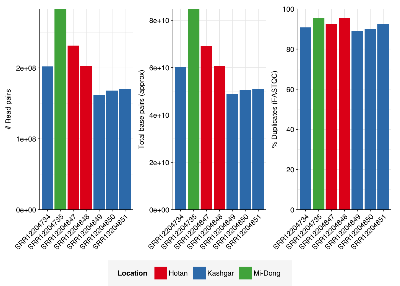
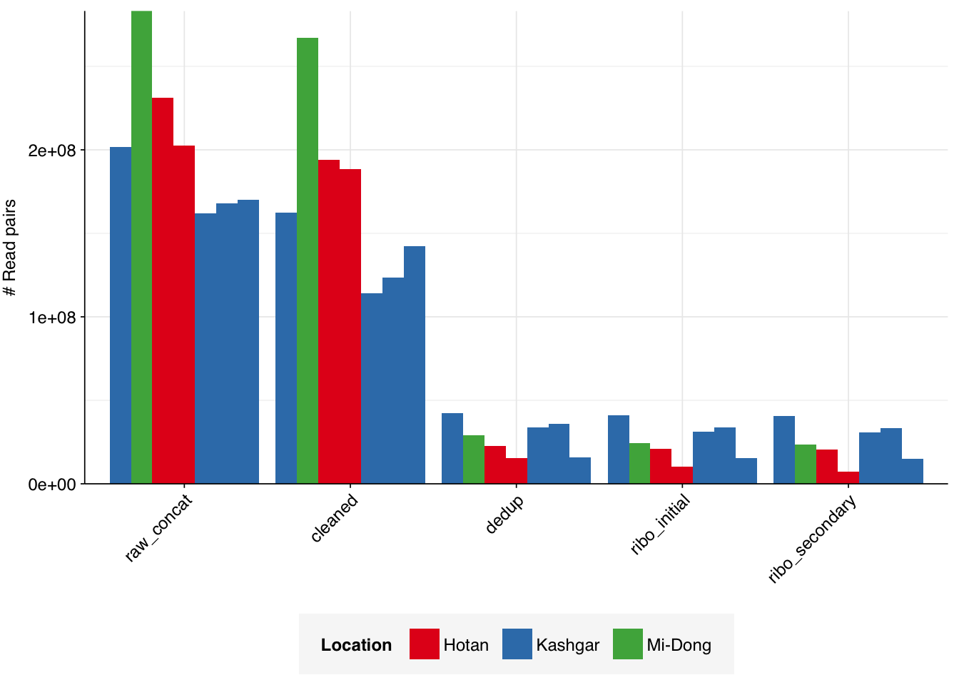
The Yang data is unusual in that it contains only a small number of samples (7 samples from 3 different locations) but each of these samples is sequenced quite deeply: the number of reads per sample varied from 162M to 283M, with an average of 203M. Taken together, the samples totaled roughly 1.4B read pairs (425 gigabases of sequence).
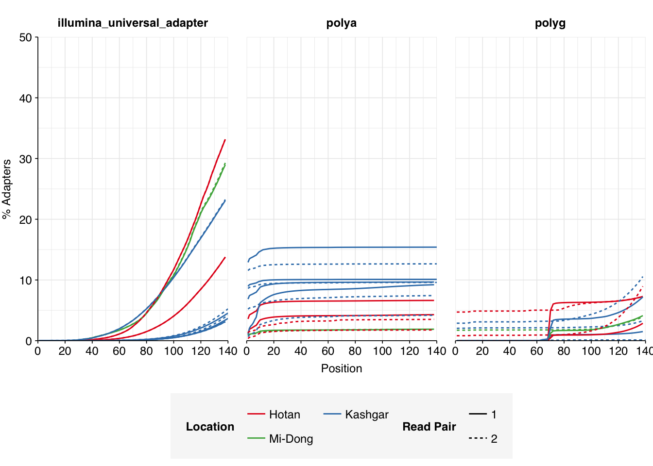
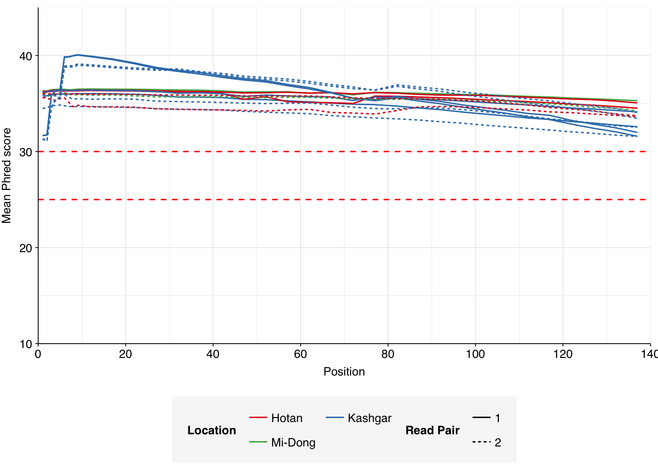
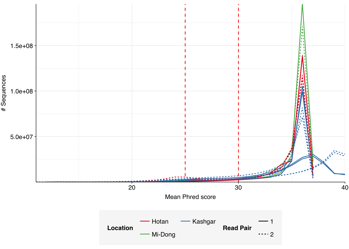
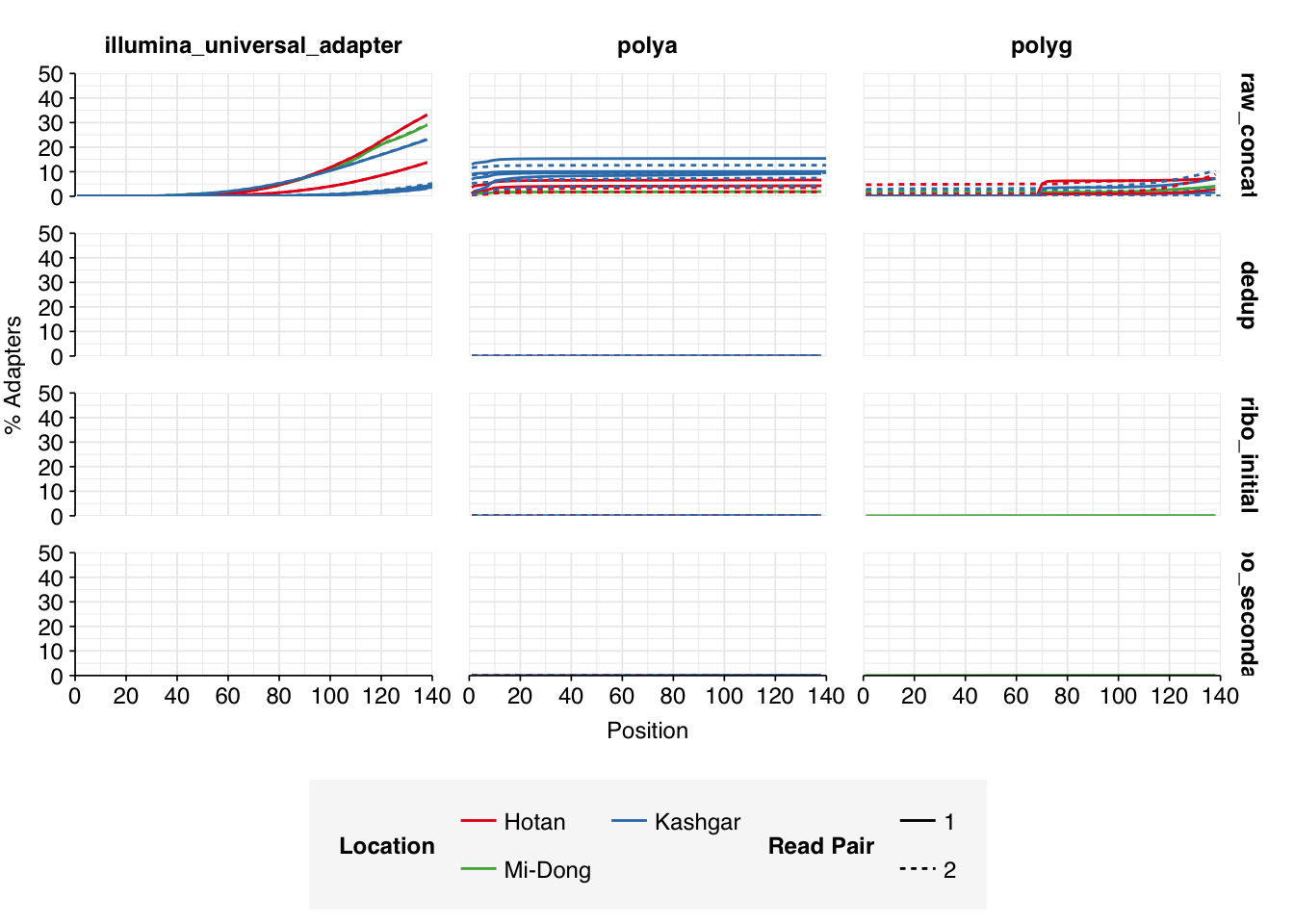
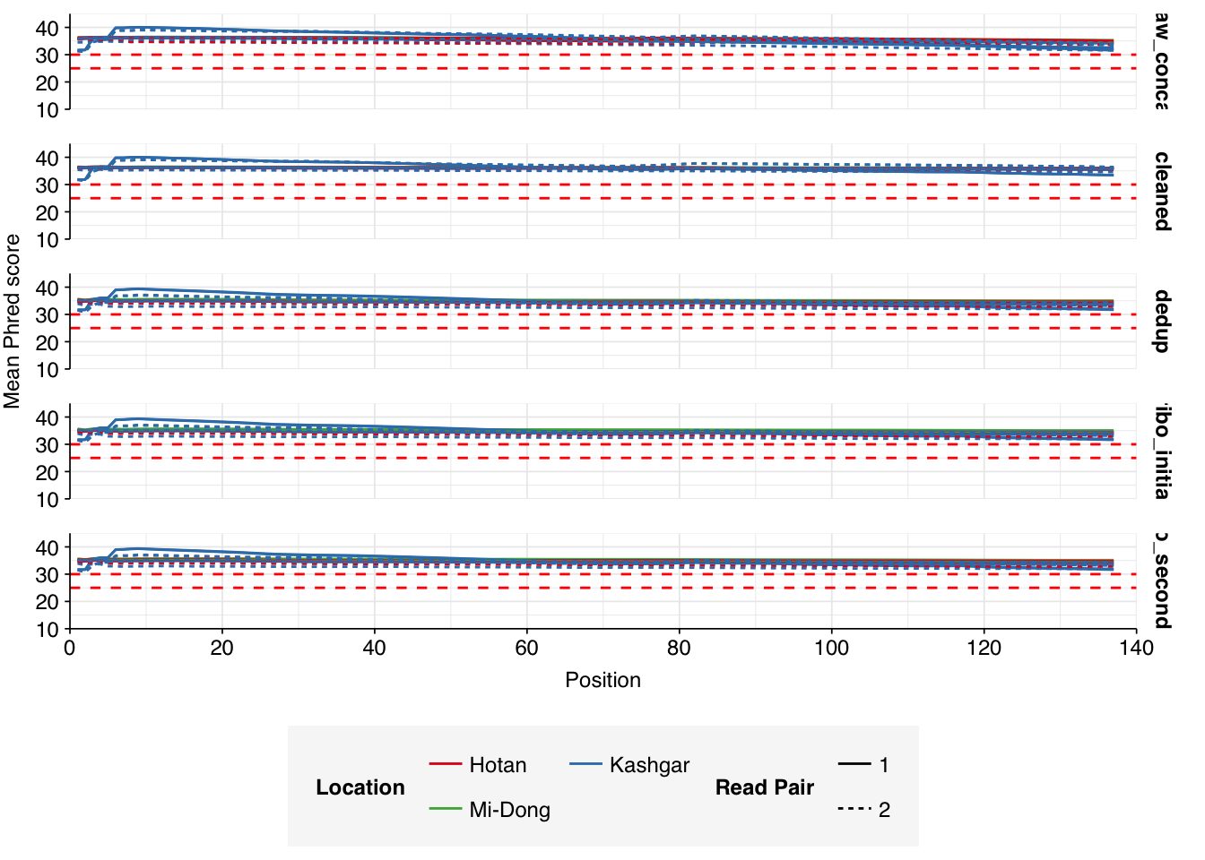
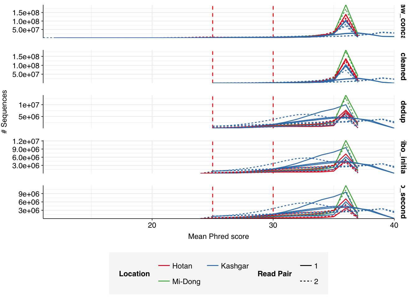
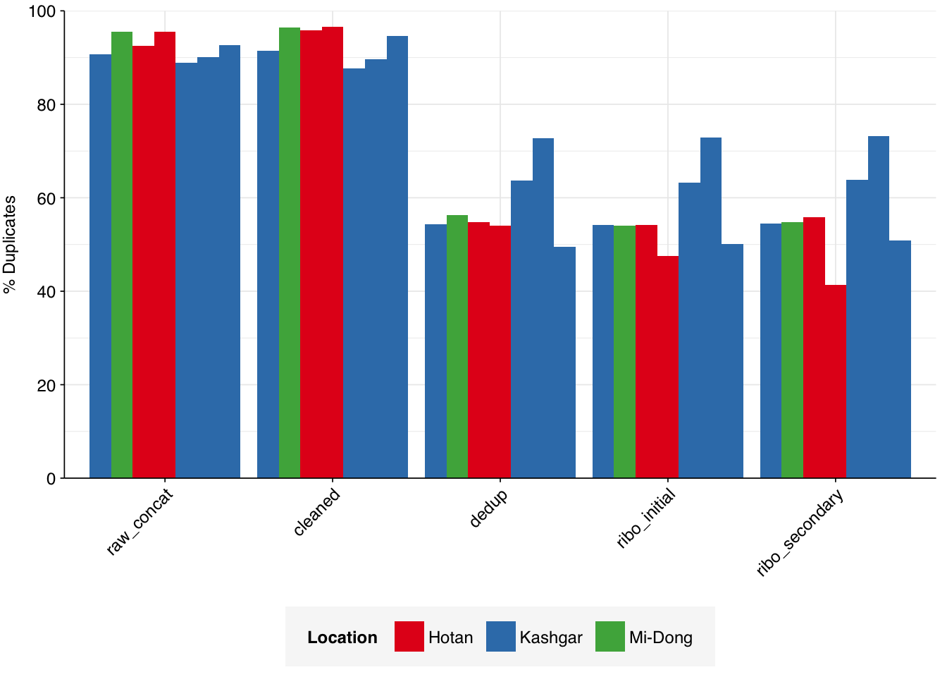
Read qualities were consistently very high, but adapter levels were also elevated. The level of sequence duplication levels was very high according to FASTQC, with a minimum of 89% across all samples, suggesting a high degree of oversequencing; perhaps unsurprising given the sheer depth of these samples.
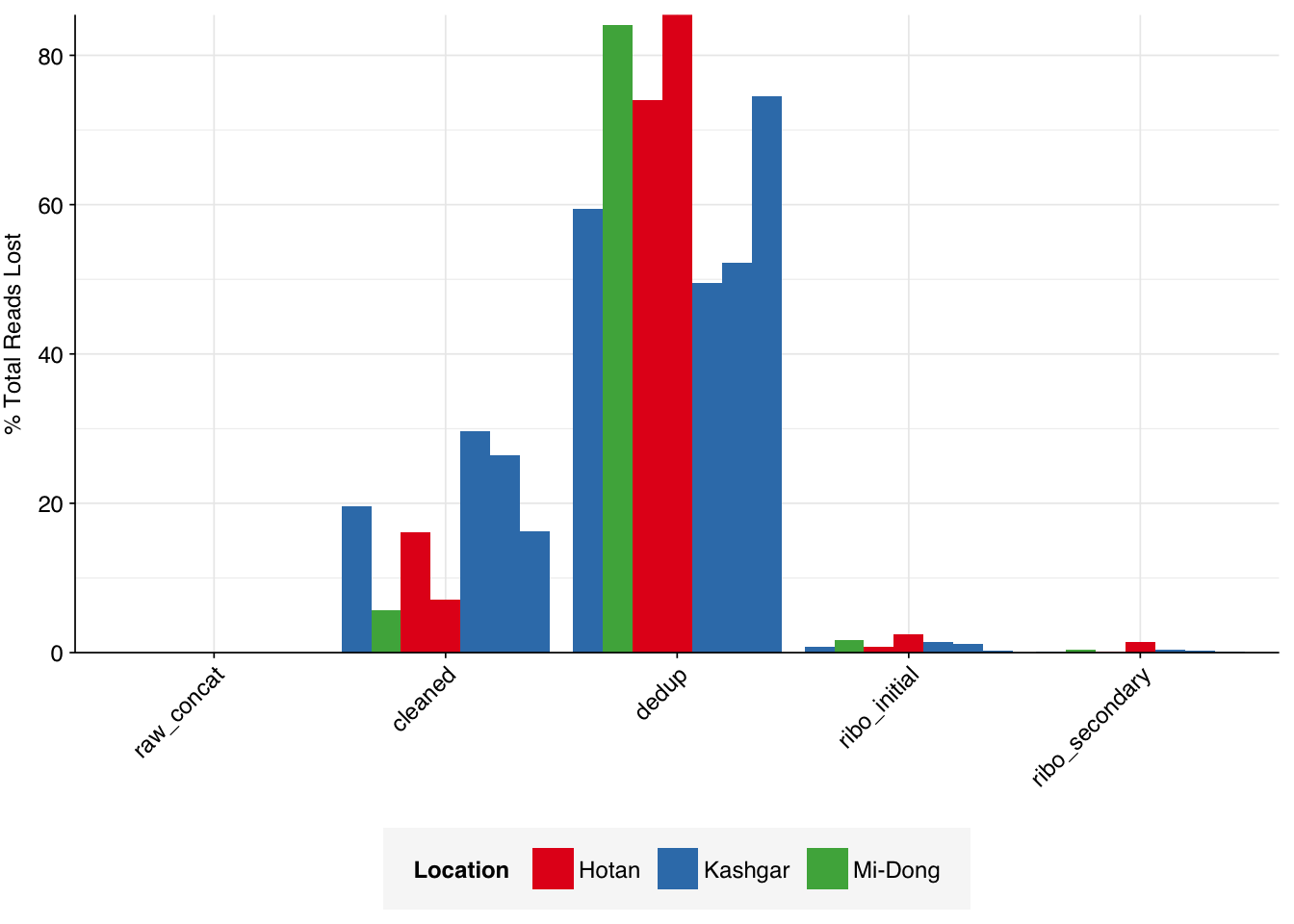
On average, cleaning & deduplication together removed about 86% of total reads from each sample, with the largest losses seen during deduplication. Only a few reads (low single-digit percentages at most) were lost during subsequent ribodepletion – a surprising finding given the apparent lack of rRNA depletion in the study methods. This makes me suspect that the methods did include rRNA depletion without mentioning it; if this isn’t the case, it suggests that the methods used by the authors might be particularly effective at removing bacteria from the sample.
# Plot relative read losses during preprocessingg_reads_rel<-ggplot(n_reads_rel, aes(x=stage, y=p_reads_lost_abs_marginal,fill=location,group=sample))+geom_col(position="dodge")+scale_fill_brewer(palette="Set1", name="Location")+scale_y_continuous("% Total Reads Lost", expand=c(0,0), labels =function(x)x*100)+theme_kitg_reads_rel
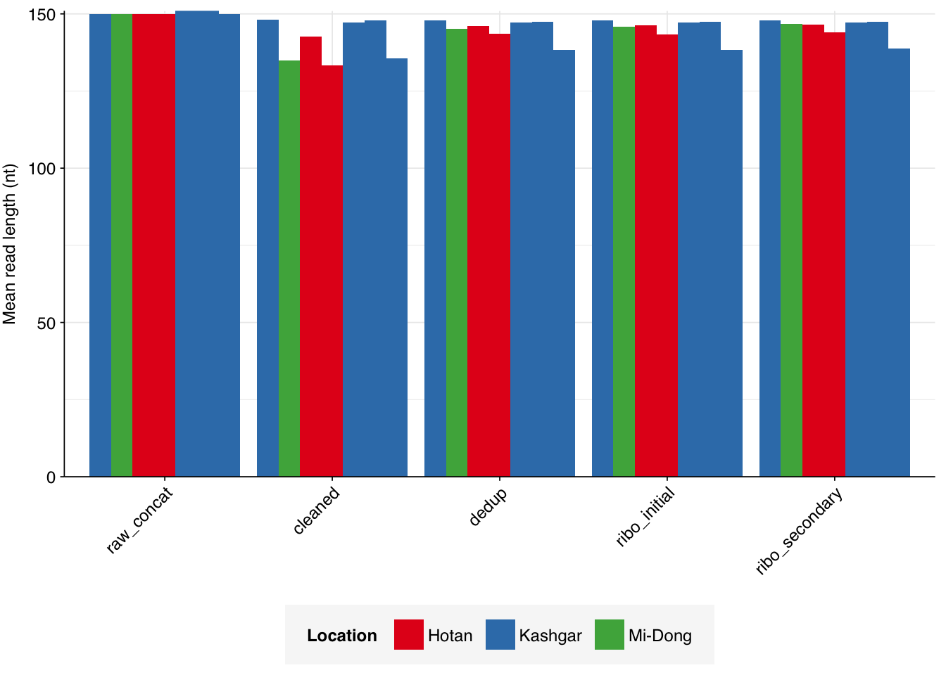
Data cleaning with FASTP was very successful at removing adapters, with very few adapter sequences found by FASTQC at any stage after the raw data. Improvements in quality were unsurprisingly minimal, given the high initial quality observed.
According to FASTQC, deduplication was only moderately effective at reducing measured duplicate levels, despite the high read losses observed. After deduplication, FASTQC-measured duplicate levels fell from an average of 92% to one of 58%:
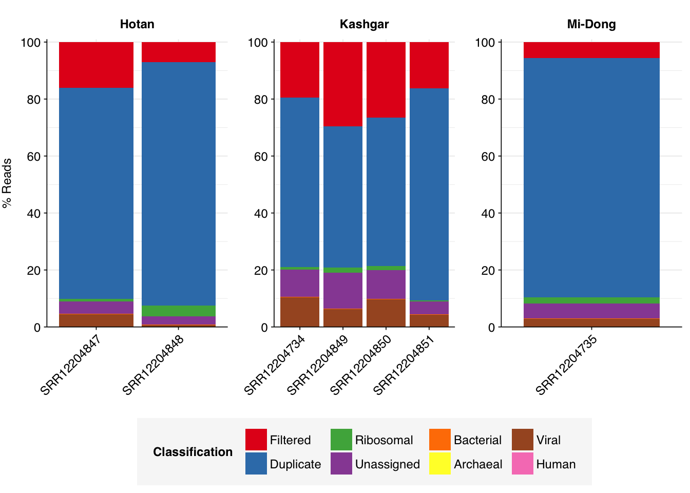
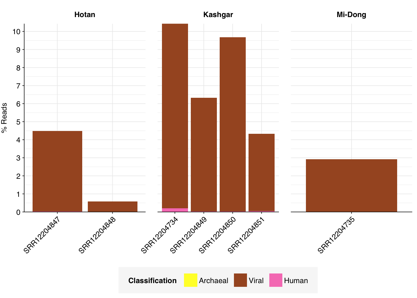
As before, to assess the high-level composition of the reads, I ran the ribodepleted files through Kraken (using the Standard 16 database) and summarized the results with Bracken. Combining these results with the read counts above gives us a breakdown of the inferred composition of the samples:
Overall, in these unenriched samples, between 89% and 95% of reads (mean 93%) are low-quality, duplicates, or unassigned. Of the remainder, 0.4-3.9% (mean 1.6%) were identified as ribosomal, and 0.06-0.22% (mean 0.13%) were otherwise classified as bacterial. The fraction of human reads ranged from 0.006-0.198% (mean 0.049%). Strikingly, those of viral reads ranged from 0.6% all the way up to 10.2% (mean 5.5%).
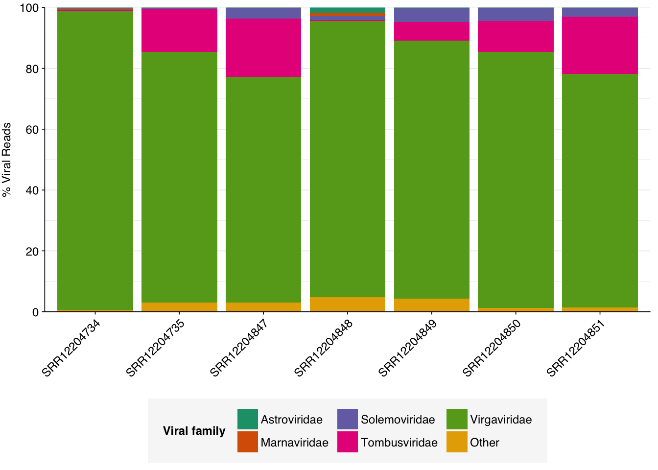
The total fraction of viral reads is strikingly high, even higher on average than for Rothman unenriched samples. As in Rothman, this is primarily accounted for by very high levels of tobamoviruses (viral family Virgaviridae), which make up 74-98% (mean 84%) of viral reads. Most of the remainder is accounted for by Tombusviridae and Solemoviridae, two other families of plant viruses. Only one family of vertebrate viruses, Astroviridae, accounted for more than 1% of viral reads in any sample.
Almost as striking as the high fraction of viral reads in these data is the extremely low prevalence of bacterial reads. For comparison, non-ribosomal bacterial reads in unenriched Crits-Christoph samples ranged from 16-20%, and in unenriched Rothman samples it ranged from 2-12%. Yang et al. are thus somehow achieving a greater than 10-fold reduction in the fraction of bacterial reads compared to other studies. Unlike the increased prevalence of viruses, this seems harder to explain away via differences in conditions on the ground. Together with the elevated viral fraction, these results suggest to me that Yang’s ideosyncratic methods are worth investigating further.
Human-infecting virus reads: validation
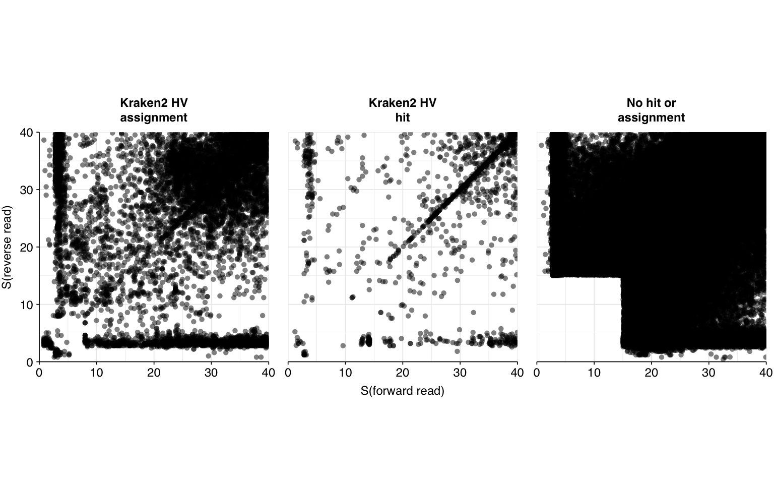
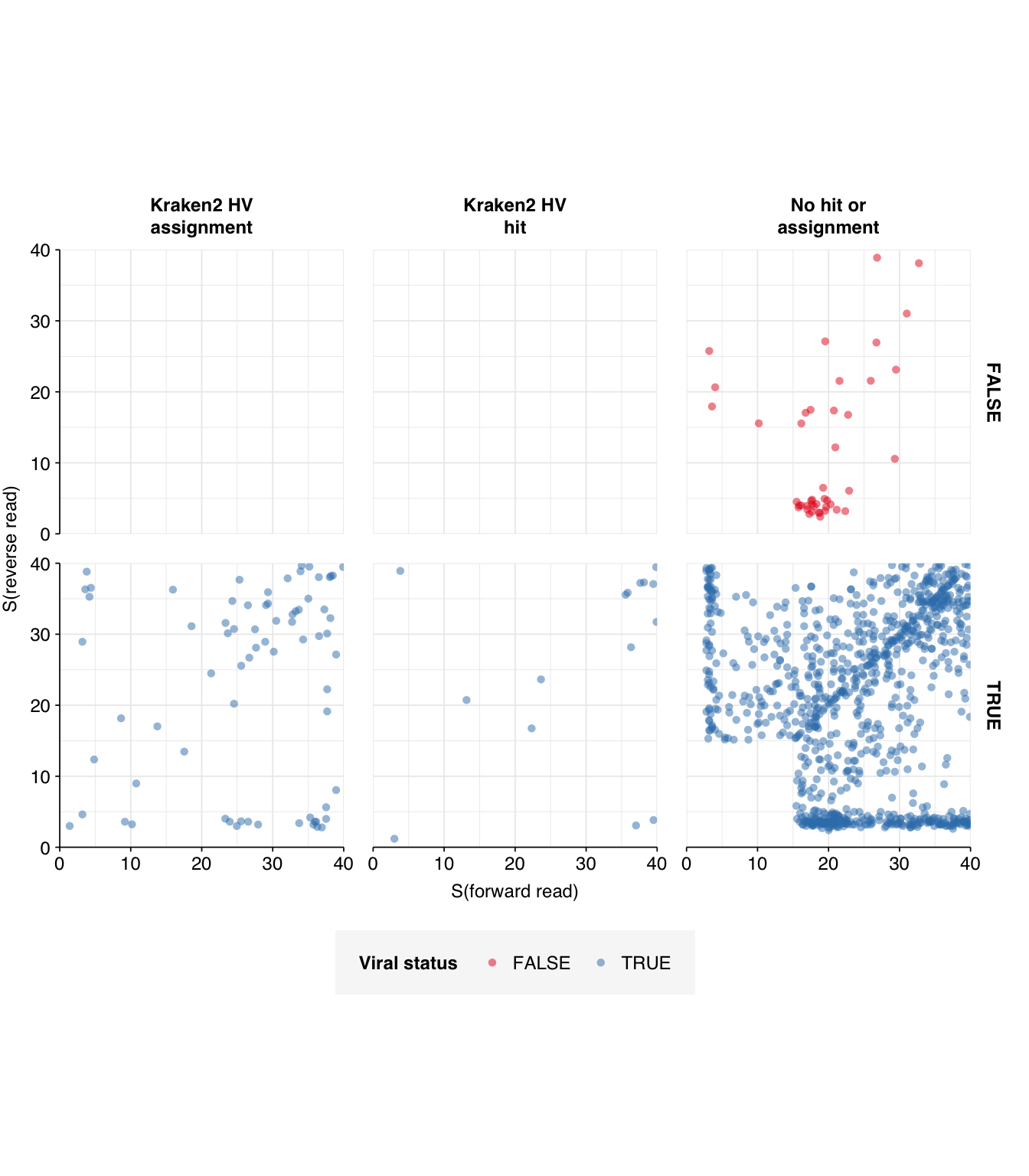
Next, I investigated the human-infecting virus read content of these unenriched samples, using a pipeline identical to that described in my entry on unenriched Rothman samples. This process identified a total of 532,583 read pairs across all samples (0.3% of surviving reads):
This is a far larger number of putative viral reads than I previously needed to analyze, and is far too many to realistically process with BLASTN. To address this problem, I selected 1% of putative viral sequences (5,326) and ran them through BLASTN in a similar manner to past datasets:
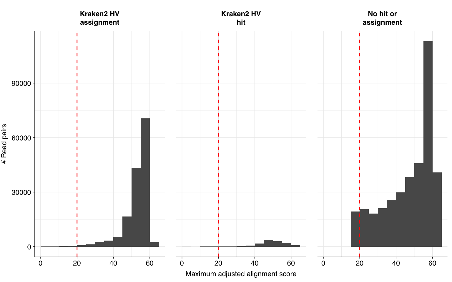
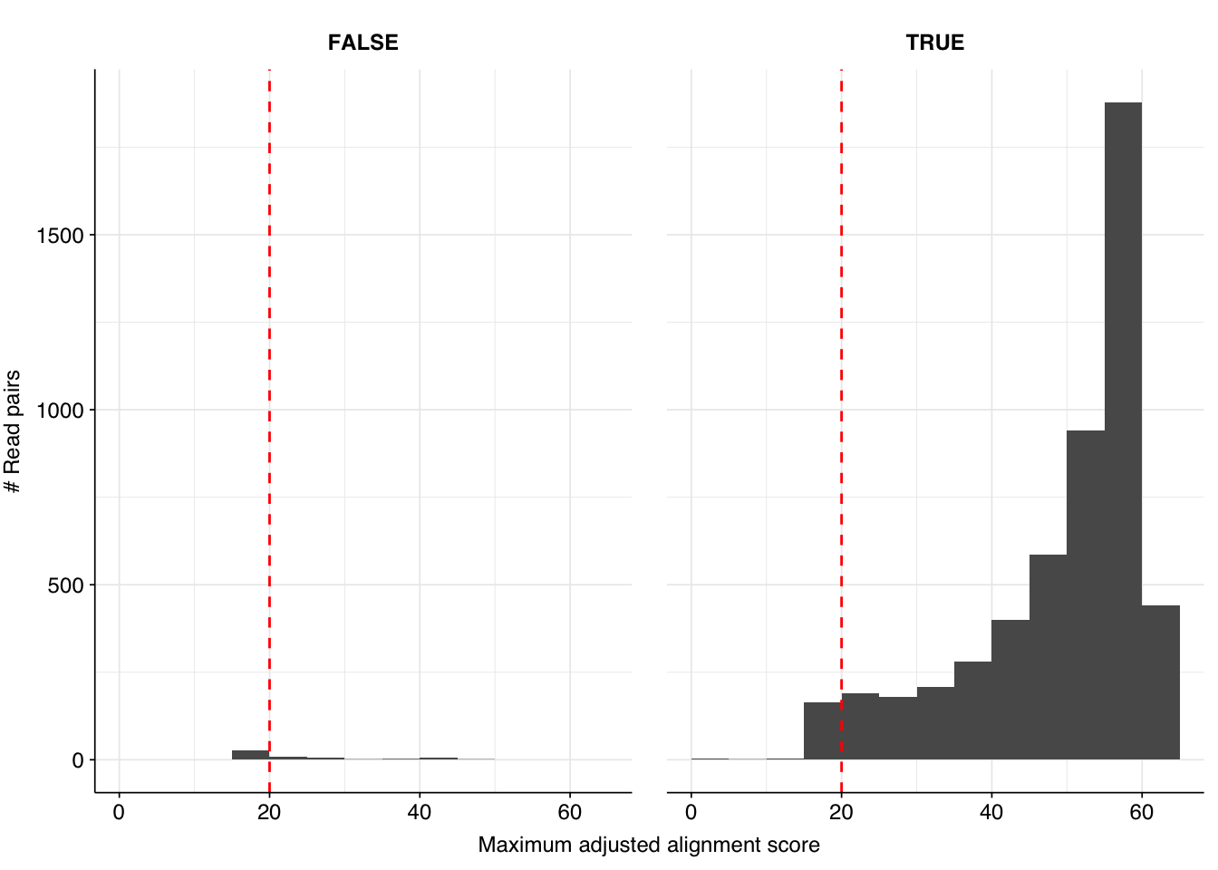
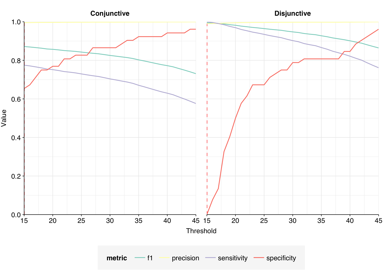
High-scoring true-positives massively outnumber false-positives, while low-scoring true-positives are fairly rare. My usual score cutoff, a disjunctive threshold at S=20, achieves a sensitivity of ~97% and an F1 score of ~98%. As such, I think this looks pretty good, and feel comfortable moving on to analyzing the entire HV dataset.
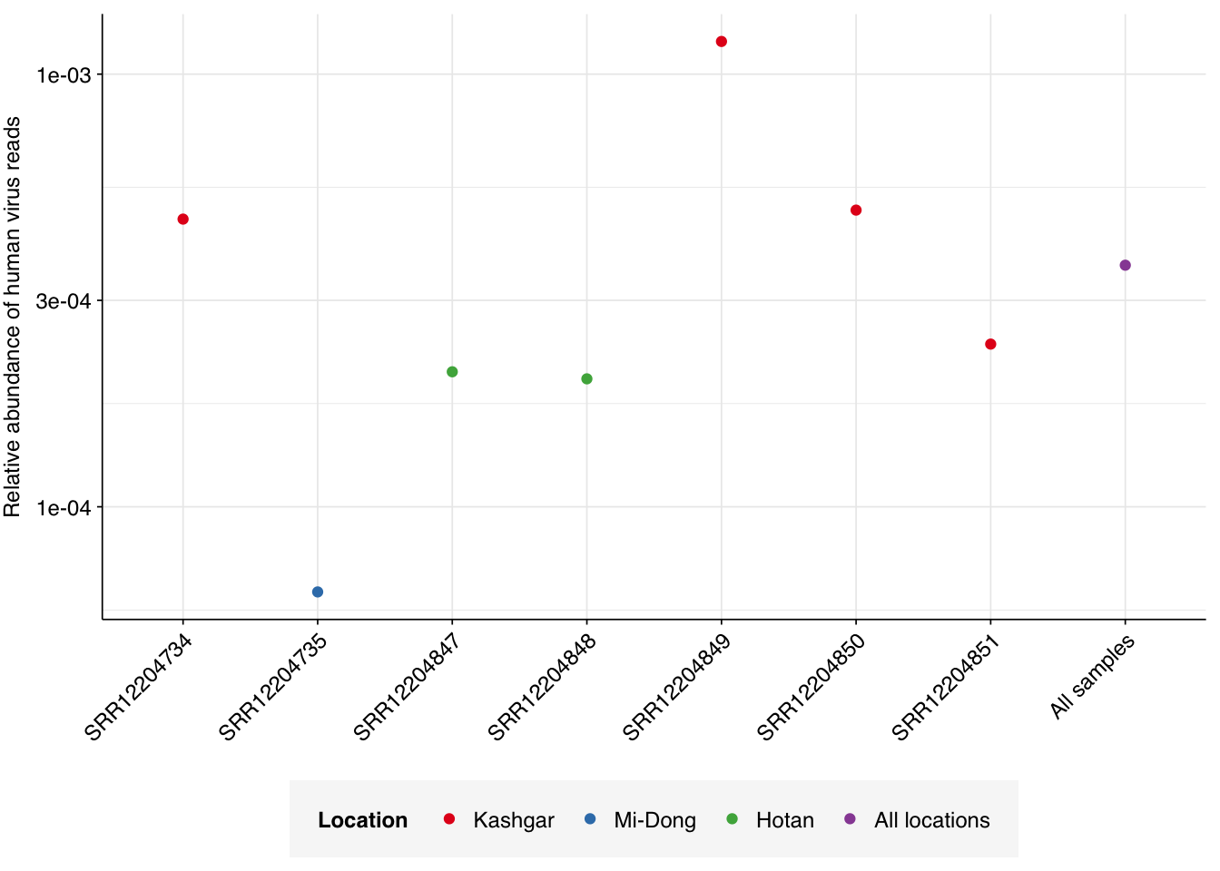
Applying a disjunctive cutoff at S=20 identifies 513,259 reads as human-viral out of 1.42B total reads, for a relative HV abundance of \(3.62 \times 10^{-4}\). This compares to \(2.0 \times 10^{-4}\) on the public dashboard, corresponding to the results for Kraken-only identification: an 80% increase, smaller than the 4-5x increases seen for Crits-Christoph and Rothman. Relative HV abundances for individual samples ranged from \(6.36 \times 10^{-5}\) to \(1.19 \times 10^{-3}\):
Code
# Visualizeg_phv_agg<-ggplot(read_counts_agg, aes(x=sample, y=p_reads_hv, color=location))+geom_point()+scale_y_log10("Relative abundance of human virus reads")+scale_color_brewer(palette ="Set1", name ="Location")+theme_kitg_phv_agg
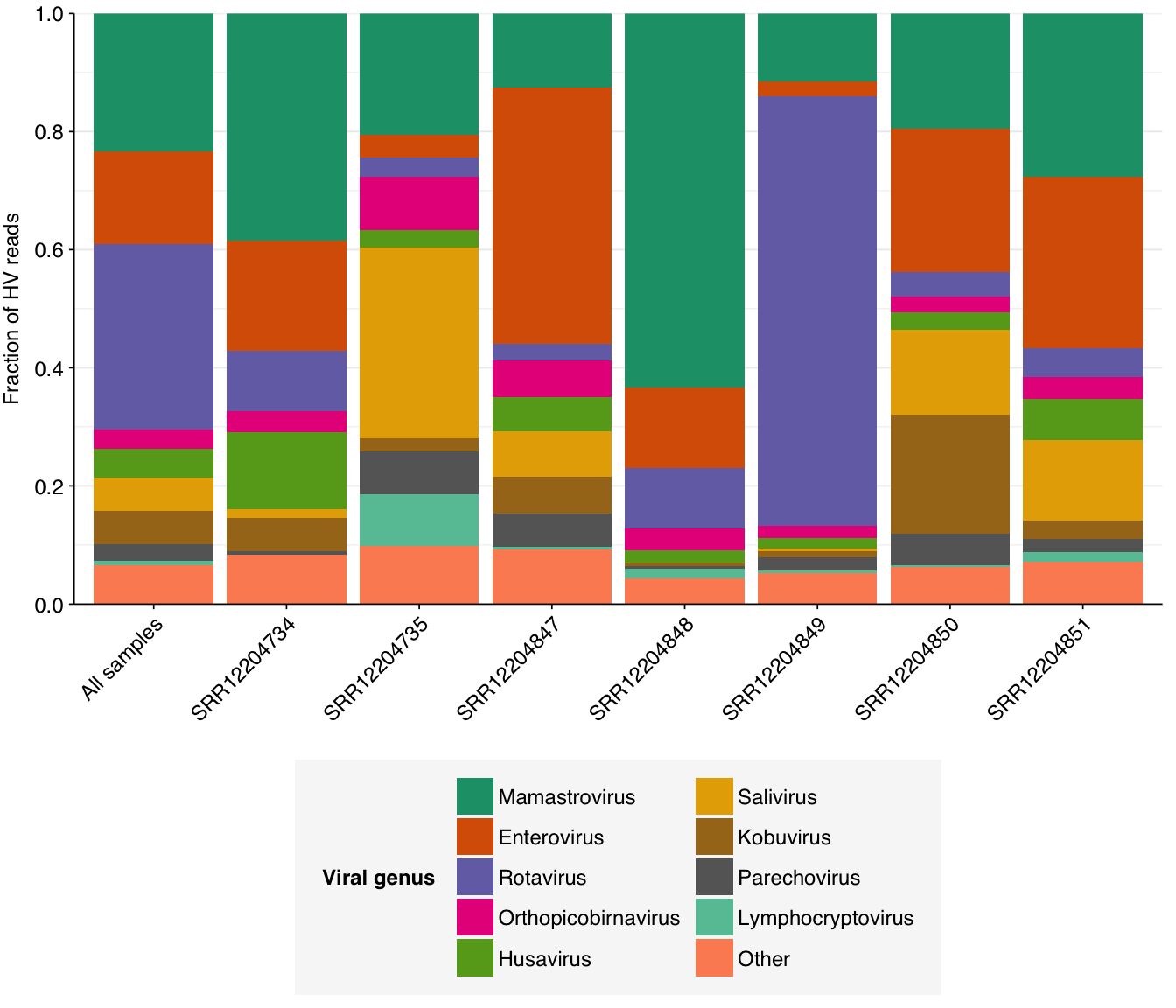
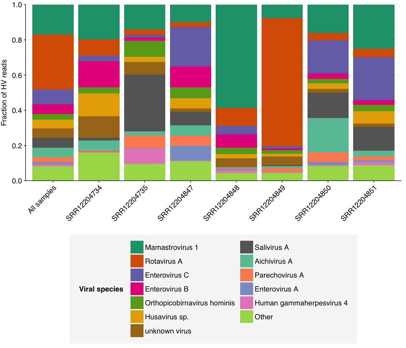
Digging into individual viruses, we see that fecal-oral viruses predominate, especially Mamastrovirus, Rotavirus, Salivirus, and fecal-oral Enterovirus species (especially Enterovirus C, which includes poliovirus):
Code
# Get viral taxon names for putative HV readsviral_taxa$name[viral_taxa$taxid==249588]<-"Mamastrovirus"viral_taxa$name[viral_taxa$taxid==194960]<-"Kobuvirus"viral_taxa$name[viral_taxa$taxid==688449]<-"Salivirus"mrg_hv_named<-mrg_hv%>%left_join(viral_taxa, by="taxid")# Discover viral species & genera for HV readsraise_rank<-function(read_db, taxid_db, out_rank="species", verbose=FALSE){# Get higher ranks than search rankranks<-c("subspecies", "species", "subgenus", "genus", "subfamily", "family", "suborder", "order", "class", "subphylum", "phylum", "kingdom", "superkingdom")rank_match<-which.max(ranks==out_rank)high_ranks<-ranks[rank_match:length(ranks)]# Merge read DB and taxid DBreads<-read_db%>%select(-parent_taxid, -rank, -name)%>%left_join(taxid_db, by="taxid")# Extract sequences that are already at appropriate rankreads_rank<-filter(reads, rank==out_rank)# Drop sequences at a higher rank and return unclassified sequencesreads_norank<-reads%>%filter(rank!=out_rank, !rank%in%high_ranks, !is.na(taxid))while(nrow(reads_norank)>0){# As long as there are unclassified sequences...# Promote read taxids and re-merge with taxid DB, then re-classify and filterreads_remaining<-reads_norank%>%mutate(taxid =parent_taxid)%>%select(-parent_taxid, -rank, -name)%>%left_join(taxid_db, by="taxid")reads_rank<-reads_remaining%>%filter(rank==out_rank)%>%bind_rows(reads_rank)reads_norank<-reads_remaining%>%filter(rank!=out_rank, !rank%in%high_ranks, !is.na(taxid))}# Finally, extract and append reads that were excluded during the processreads_dropped<-reads%>%filter(!seq_id%in%reads_rank$seq_id)reads_out<-reads_rank%>%bind_rows(reads_dropped)%>%select(-parent_taxid, -rank, -name)%>%left_join(taxid_db, by="taxid")return(reads_out)}hv_reads_species<-raise_rank(mrg_hv_named, viral_taxa, "species")hv_reads_genera<-raise_rank(mrg_hv_named, viral_taxa, "genus")
# Compute ranks for species and genera and restrict to high-ranking taxamax_rank_species<-5max_rank_genera<-5hv_species_counts_ranked<-hv_species_counts_agg%>%group_by(sample)%>%mutate(rank =rank(desc(n_reads_hv), ties.method="max"), highrank =rank<=max_rank_species)%>%group_by(name)%>%mutate(highrank_any =any(highrank), name_display =ifelse(highrank_any, name, "Other"))%>%group_by(name_display)%>%mutate(mean_rank =mean(rank))%>%arrange(mean_rank)%>%ungroup%>%mutate(name_display =fct_inorder(name_display))hv_genera_counts_ranked<-hv_genera_counts_agg%>%group_by(sample)%>%mutate(rank =rank(desc(n_reads_hv), ties.method="max"), highrank =rank<=max_rank_genera)%>%group_by(name)%>%mutate(highrank_any =any(highrank), name_display =ifelse(highrank_any, name, "Other"))%>%group_by(name_display)%>%mutate(mean_rank =mean(rank))%>%arrange(mean_rank)%>%ungroup%>%mutate(name_display =fct_inorder(name_display))# Plot compositionpalette_rank<-c(brewer.pal(8, "Dark2"), brewer.pal(8, "Set2"))g_vcomp_genera<-ggplot(hv_genera_counts_ranked, aes(x=sample, y=n_reads_hv, fill=name_display))+geom_col(position ="fill")+scale_fill_manual(values =palette_rank, name ="Viral genus")+scale_y_continuous(name ="Fraction of HV reads", breaks =seq(0,1,0.2), expand =c(0,0))+guides(fill =guide_legend(nrow=5))+theme_kitg_vcomp_species<-ggplot(hv_species_counts_ranked, aes(x=sample, y=n_reads_hv, fill=name_display))+geom_col(position ="fill")+scale_fill_manual(values =palette_rank, name ="Viral species")+scale_y_continuous(name ="Fraction of HV reads", breaks =seq(0,1,0.2), expand =c(0,0))+guides(fill =guide_legend(nrow=7))+theme_kitg_vcomp_genera
Code
g_vcomp_species
These results are consistent with what’s been observed before, e.g. in the P2RA preprint and public dashboard.
Conclusion
I analyzed Yang et al. for two reasons: first, because it’s included in the P2RA dataset that we’re currently reanalyzing, and second, because it has the highest relative abundance of both total and human-infecting viruses of any wastewater study we’ve looked at so far. Having done this analysis, the key question to ask is: is this elevated viral abundance a consequence of the unusual sample-processing methods employed by the authors, or the region in which samples were collected? Both are plausible: the processing methods used in this paper are distinct from any other paper we’ve looked at, which makes it possible that they are significantly superior; on the other hand, it’s also plausible that the methods are comparable in efficacy to more standard approaches, and the difference arises from a genuinely elevated level of viruses in Xinjiang compared to e.g. California (for Rothman and Crits-Christoph).
The analyses conducted here aren’t able to give a dispositive answer to that question, but they are suggestive. The fact that human-infecting viruses are strongly dominated by fecal-oral species is consistent with the elevated-infection theory, as these are the kinds of viruses I’d most expect to be elevated in a poorer region of the world compared to a rich one. On the other hand, the fact that total viruses (including plant viruses) are also elevated points in the other direction; I don’t see any obvious reason why we’d expect more tobamoviruses in Xinjiang than California.
Most compellingly, from my perspective, is the very low fraction of bacterial and ribosomal reads found in the Yang data compared to other datasets I’ve analyzed. The methods make no mention of rRNA depletion prior to sequencing; even if this was conducted without being mentioned, that still doesn’t explain the very low level of non-ribosomal bacterial reads. In general, I’d expect a region with elevated enteric viral pathogens to also show elevated enteric bacterial pathogens, so this absence is difficult to explain with a catchment-based theory. Instead, it points towards the viral enrichment protocols used by this study as potentially achieving genuinely better results than other methods we’ve tried.
This certainly isn’t conclusive evidence, or close to it. However, based on these results, I’d be very interested in learning more about the details of Yang et al’s approach to viral enrichment, and to see it tried by another group in a different context to see if these impressive results can be replicated.
Source Code
---title: "Workflow analysis of Yang et al. (2020)"subtitle: "Wastewater from Xinjiang."author: "Will Bradshaw"date: 2024-03-16format: html: code-fold: true code-tools: true code-link: true df-print: pagededitor: visualtitle-block-banner: black---```{r}#| label: load-packages#| include: falselibrary(tidyverse)library(cowplot)library(patchwork)library(fastqcr)library(RColorBrewer)source("../scripts/aux_plot-theme.R")theme_base <- theme_base +theme(aspect.ratio =NULL)theme_kit <- theme_base +theme(axis.text.x =element_text(hjust =1, angle =45),axis.title.x =element_blank(),)tnl <-theme(legend.position ="none")```As we work on expanding and updating the [P2RA preprint](https://doi.org/10.1101/2023.12.22.23300450) for publication, I'm working on running the relevant datasets through my pipeline to compare the results to those from the original Kraken-based approach. I began by processing [Yang et al. (2020)](https://doi.org/10.1016/j.scitotenv.2020.142322), a study that carried out RNA viral metagenomics on raw sewage samples from Xinjiang, China.The study collected 7 1L grab samples of raw sewage from the inlets of three WWTPs in Xinjiang, and processed them using an "anion filter membrane absorption" method quite distinct from the [other](https://data.securebio.org/wills-public-notebook/notebooks/2024-02-04_crits-christoph-1.html)[studies](https://data.securebio.org/wills-public-notebook/notebooks/2024-02-27_rothman-1.html) I've looked at so far:1. Initially, samples were centrifuged to pellet cells and debris.2. The supernatant was treated with magnesium chloride and HCl, then filtered through a mixed cellulose ester membrane filter, **discarding the filtrate**.3. Material was then eluted from the filters by ultrasonication with 3% beef extract, before going a second filtering step using a 0.22um filter, this time retaining the filtrate.4. Next, the samples underwent RNA extraction using the QIAamp viral RNA Mini Kit.5. Finally, sequencing libraries were generated using KAPA Hyper Prep Kit. No mention is made of rRNA depletion or panel enrichment.This study is of particular interest because previous analysis found that the MGS data it generated contains a particularly high fraction of both total viruses and human-infecting viruses. It would be good to know whether this is attributable to the fact that the authors used an unusual method, or if it's the result of genuine differences on the ground (e.g. an elevated prevalence of enteric disease compared to the USA).# The raw dataThe Yang data is unusual in that it contains only a small number of samples (7 samples from 3 different locations) but each of these samples is sequenced quite deeply: the number of reads per sample varied from 162M to 283M, with an average of 203M. Taken together, the samples totaled roughly 1.4B read pairs (425 gigabases of sequence).Read qualities were consistently very high, but adapter levels were also elevated. The level of sequence duplication levels was very high according to FASTQC, with a minimum of 89% across all samples, suggesting a high degree of oversequencing; perhaps unsurprising given the sheer depth of these samples.```{r}#| fig-height: 5#| warning: false# Data input pathsdata_dir <-"../data/2024-03-15_yang/"libraries_path <-file.path(data_dir, "sample-metadata.csv")basic_stats_path <-file.path(data_dir, "qc_basic_stats.tsv")adapter_stats_path <-file.path(data_dir, "qc_adapter_stats.tsv")quality_base_stats_path <-file.path(data_dir, "qc_quality_base_stats.tsv")quality_seq_stats_path <-file.path(data_dir, "qc_quality_sequence_stats.tsv")# Import libraries and extract metadata from sample nameslibraries <-read_csv(libraries_path, show_col_types =FALSE)# Import QC datastages <-c("raw_concat", "cleaned", "dedup", "ribo_initial", "ribo_secondary")basic_stats <-read_tsv(basic_stats_path, show_col_types =FALSE) %>%# mutate(sample = sub("_2$", "", sample)) %>%inner_join(libraries, by="sample") %>%mutate(stage =factor(stage, levels = stages),sample =fct_inorder(sample))adapter_stats <-read_tsv(adapter_stats_path, show_col_types =FALSE) %>%mutate(sample =sub("_2$", "", sample)) %>%inner_join(libraries, by="sample") %>%mutate(stage =factor(stage, levels = stages),read_pair =fct_inorder(as.character(read_pair)))quality_base_stats <-read_tsv(quality_base_stats_path, show_col_types =FALSE) %>%# mutate(sample = sub("_2$", "", sample)) %>%inner_join(libraries, by="sample") %>%mutate(stage =factor(stage, levels = stages),read_pair =fct_inorder(as.character(read_pair)))quality_seq_stats <-read_tsv(quality_seq_stats_path, show_col_types =FALSE) %>%# mutate(sample = sub("_2$", "", sample)) %>%inner_join(libraries, by="sample") %>%mutate(stage =factor(stage, levels = stages),read_pair =fct_inorder(as.character(read_pair)))# Filter to raw databasic_stats_raw <- basic_stats %>%filter(stage =="raw_concat")adapter_stats_raw <- adapter_stats %>%filter(stage =="raw_concat")quality_base_stats_raw <- quality_base_stats %>%filter(stage =="raw_concat")quality_seq_stats_raw <- quality_seq_stats %>%filter(stage =="raw_concat")# Visualize basic statsg_nreads_raw <-ggplot(basic_stats_raw, aes(x=sample, y=n_read_pairs, fill=location)) +geom_col(position="dodge") +scale_y_continuous(name="# Read pairs", expand=c(0,0)) +scale_fill_brewer(palette="Set1", name="Location") + theme_kitlegend_location <-get_legend(g_nreads_raw)g_nreads_raw_2 <- g_nreads_raw +theme(legend.position ="none")g_nbases_raw <-ggplot(basic_stats_raw, aes(x=sample, y=n_bases_approx, fill=location)) +geom_col(position="dodge") +scale_y_continuous(name="Total base pairs (approx)", expand=c(0,0)) +scale_fill_brewer(palette="Set1", name="Location") + theme_kit +theme(legend.position ="none")g_ndup_raw <-ggplot(basic_stats_raw, aes(x=sample, y=percent_duplicates, fill=location)) +geom_col(position="dodge") +scale_y_continuous(name="% Duplicates (FASTQC)", expand=c(0,0), limits =c(0,100), breaks =seq(0,100,20)) +scale_fill_brewer(palette="Set1", name="Location") + theme_kit +theme(legend.position ="none")g_basic_raw <-plot_grid(g_nreads_raw_2 + g_nbases_raw + g_ndup_raw, legend_location, ncol =1, rel_heights =c(1,0.1))g_basic_raw# Visualize adaptersg_adapters_raw <-ggplot(adapter_stats_raw, aes(x=position, y=pc_adapters, color=location, linetype = read_pair, group=interaction(sample, read_pair))) +geom_line() +scale_color_brewer(palette ="Set1", name ="Location") +scale_linetype_discrete(name ="Read Pair") +scale_y_continuous(name="% Adapters", limits=c(0,50),breaks =seq(0,50,10), expand=c(0,0)) +scale_x_continuous(name="Position", limits=c(0,140),breaks=seq(0,140,20), expand=c(0,0)) +guides(color=guide_legend(nrow=2,byrow=TRUE),linetype =guide_legend(nrow=2,byrow=TRUE)) +facet_wrap(~adapter) + theme_baseg_adapters_raw# Visualize qualityg_quality_base_raw <-ggplot(quality_base_stats_raw, aes(x=position, y=mean_phred_score, color=location, linetype = read_pair, group=interaction(sample,read_pair))) +geom_hline(yintercept=25, linetype="dashed", color="red") +geom_hline(yintercept=30, linetype="dashed", color="red") +geom_line() +scale_color_brewer(palette ="Set1", name ="Location") +scale_linetype_discrete(name ="Read Pair") +scale_y_continuous(name="Mean Phred score", expand=c(0,0), limits=c(10,45)) +scale_x_continuous(name="Position", limits=c(0,140),breaks=seq(0,140,20), expand=c(0,0)) +guides(color=guide_legend(nrow=2,byrow=TRUE),linetype =guide_legend(nrow=2,byrow=TRUE)) + theme_baseg_quality_seq_raw <-ggplot(quality_seq_stats_raw, aes(x=mean_phred_score, y=n_sequences, color=location, linetype = read_pair, group=interaction(sample,read_pair))) +geom_vline(xintercept=25, linetype="dashed", color="red") +geom_vline(xintercept=30, linetype="dashed", color="red") +geom_line() +scale_color_brewer(palette ="Set1", name ="Location") +scale_linetype_discrete(name ="Read Pair") +scale_x_continuous(name="Mean Phred score", expand=c(0,0)) +scale_y_continuous(name="# Sequences", expand=c(0,0)) +guides(color=guide_legend(nrow=2,byrow=TRUE),linetype =guide_legend(nrow=2,byrow=TRUE)) + theme_baseg_quality_base_rawg_quality_seq_raw```# Preprocessing```{r}n_reads_rel <- basic_stats %>%select(sample, location, stage, percent_duplicates, n_read_pairs) %>%group_by(sample, location) %>%arrange(sample, location, stage) %>%mutate(p_reads_retained = n_read_pairs /lag(n_read_pairs),p_reads_lost =1- p_reads_retained,p_reads_retained_abs = n_read_pairs / n_read_pairs[1],p_reads_lost_abs =1-p_reads_retained_abs,p_reads_lost_abs_marginal = p_reads_lost_abs -lag(p_reads_lost_abs))```On average, cleaning & deduplication together removed about 86% of total reads from each sample, with the largest losses seen during deduplication. Only a few reads (low single-digit percentages at most) were lost during subsequent ribodepletion – a surprising finding given the apparent lack of rRNA depletion in the study methods. This makes me suspect that the methods did include rRNA depletion without mentioning it; if this isn't the case, it suggests that the methods used by the authors might be particularly effective at removing bacteria from the sample.```{r}#| warning: false# Plot reads over preprocessingg_reads_stages <-ggplot(basic_stats, aes(x=stage, y=n_read_pairs,fill=location,group=sample)) +geom_col(position="dodge") +scale_fill_brewer(palette="Set1", name="Location") +scale_y_continuous("# Read pairs", expand=c(0,0)) + theme_kitg_reads_stages# Plot relative read losses during preprocessingg_reads_rel <-ggplot(n_reads_rel, aes(x=stage, y=p_reads_lost_abs_marginal,fill=location,group=sample)) +geom_col(position="dodge") +scale_fill_brewer(palette="Set1", name="Location") +scale_y_continuous("% Total Reads Lost", expand=c(0,0), labels =function(x) x*100) + theme_kitg_reads_rel```Data cleaning with FASTP was very successful at removing adapters, with very few adapter sequences found by FASTQC at any stage after the raw data. Improvements in quality were unsurprisingly minimal, given the high initial quality observed.```{r}#| warning: false# Visualize adaptersg_adapters <-ggplot(adapter_stats, aes(x=position, y=pc_adapters, color=location, linetype = read_pair, group=interaction(sample, read_pair))) +geom_line() +scale_color_brewer(palette ="Set1", name ="Location") +scale_linetype_discrete(name ="Read Pair") +scale_y_continuous(name="% Adapters", limits=c(0,50),breaks =seq(0,50,10), expand=c(0,0)) +scale_x_continuous(name="Position", limits=c(0,140),breaks=seq(0,140,20), expand=c(0,0)) +guides(color=guide_legend(nrow=2,byrow=TRUE),linetype =guide_legend(nrow=2,byrow=TRUE)) +facet_grid(stage~adapter) + theme_baseg_adapters# Visualize qualityg_quality_base <-ggplot(quality_base_stats, aes(x=position, y=mean_phred_score, color=location, linetype = read_pair, group=interaction(sample,read_pair))) +geom_hline(yintercept=25, linetype="dashed", color="red") +geom_hline(yintercept=30, linetype="dashed", color="red") +geom_line() +scale_color_brewer(palette ="Set1", name ="Location") +scale_linetype_discrete(name ="Read Pair") +scale_y_continuous(name="Mean Phred score", expand=c(0,0), limits=c(10,45)) +scale_x_continuous(name="Position", limits=c(0,140),breaks=seq(0,140,20), expand=c(0,0)) +guides(color=guide_legend(nrow=2,byrow=TRUE),linetype =guide_legend(nrow=2,byrow=TRUE)) +facet_grid(stage~.) + theme_baseg_quality_seq <-ggplot(quality_seq_stats, aes(x=mean_phred_score, y=n_sequences, color=location, linetype = read_pair, group=interaction(sample,read_pair))) +geom_vline(xintercept=25, linetype="dashed", color="red") +geom_vline(xintercept=30, linetype="dashed", color="red") +geom_line() +scale_color_brewer(palette ="Set1", name ="Location") +scale_linetype_discrete(name ="Read Pair") +scale_x_continuous(name="Mean Phred score", expand=c(0,0)) +scale_y_continuous(name="# Sequences", expand=c(0,0)) +guides(color=guide_legend(nrow=2,byrow=TRUE),linetype =guide_legend(nrow=2,byrow=TRUE)) +facet_grid(stage~., scales="free_y") + theme_baseg_quality_baseg_quality_seq```According to FASTQC, deduplication was only moderately effective at reducing measured duplicate levels, despite the high read losses observed. After deduplication, FASTQC-measured duplicate levels fell from an average of 92% to one of 58%:```{r}g_dup_stages <-ggplot(basic_stats, aes(x=stage, y=percent_duplicates, fill=location, group=sample)) +geom_col(position="dodge") +scale_fill_brewer(palette ="Set1", name="Location") +scale_y_continuous("% Duplicates", limits=c(0,100), breaks=seq(0,100,20), expand=c(0,0)) + theme_kitg_readlen_stages <-ggplot(basic_stats, aes(x=stage, y=mean_seq_len, fill=location, group=sample)) +geom_col(position="dodge") +scale_fill_brewer(palette ="Set1", name="Location") +scale_y_continuous("Mean read length (nt)", expand=c(0,0)) + theme_kitlegend_loc <-get_legend(g_dup_stages)g_dup_stagesg_readlen_stages```# High-level compositionAs before, to assess the high-level composition of the reads, I ran the ribodepleted files through Kraken (using the Standard 16 database) and summarized the results with Bracken. Combining these results with the read counts above gives us a breakdown of the inferred composition of the samples:```{r}# Import Bracken databracken_path <-file.path(data_dir, "bracken_counts.tsv")bracken <-read_tsv(bracken_path, show_col_types =FALSE)total_assigned <- bracken %>%group_by(sample) %>%summarize(name ="Total",kraken_assigned_reads =sum(kraken_assigned_reads),added_reads =sum(added_reads),new_est_reads =sum(new_est_reads),fraction_total_reads =sum(fraction_total_reads))bracken_spread <- bracken %>%select(name, sample, new_est_reads) %>%mutate(name =tolower(name)) %>%pivot_wider(id_cols ="sample", names_from ="name", values_from ="new_est_reads")# Count readsread_counts_preproc <- basic_stats %>%select(sample, location, stage, n_read_pairs) %>%pivot_wider(id_cols =c("sample", "location"), names_from="stage", values_from="n_read_pairs")read_counts <- read_counts_preproc %>%inner_join(total_assigned %>%select(sample, new_est_reads), by ="sample") %>%rename(assigned = new_est_reads) %>%inner_join(bracken_spread, by="sample")# Assess compositionread_comp <-transmute(read_counts, sample=sample, location=location,n_filtered = raw_concat-cleaned,n_duplicate = cleaned-dedup,n_ribosomal = (dedup-ribo_initial) + (ribo_initial-ribo_secondary),n_unassigned = ribo_secondary-assigned,n_bacterial = bacteria,n_archaeal = archaea,n_viral = viruses,n_human = eukaryota)read_comp_long <-pivot_longer(read_comp, -(sample:location), names_to ="classification",names_prefix ="n_", values_to ="n_reads") %>%mutate(classification =fct_inorder(str_to_sentence(classification))) %>%group_by(sample) %>%mutate(p_reads = n_reads/sum(n_reads))read_comp_summ <- read_comp_long %>%group_by(location, classification) %>%summarize(n_reads =sum(n_reads), .groups ="drop_last") %>%mutate(n_reads =replace_na(n_reads,0),p_reads = n_reads/sum(n_reads),pc_reads = p_reads*100)# Plot overall compositiong_comp <-ggplot(read_comp_long, aes(x=sample, y=p_reads, fill=classification)) +geom_col(position ="stack") +scale_y_continuous(name ="% Reads", limits =c(0,1.01), breaks =seq(0,1,0.2),expand =c(0,0), labels =function(x) x*100) +scale_fill_brewer(palette ="Set1", name ="Classification") +facet_wrap(.~location, scales="free") + theme_kitg_comp# Plot composition of minor componentsread_comp_minor <- read_comp_long %>%filter(classification %in%c("Archaeal", "Viral", "Human", "Other"))palette_minor <-brewer.pal(9, "Set1")[6:9]g_comp_minor <-ggplot(read_comp_minor, aes(x=sample, y=p_reads, fill=classification)) +geom_col(position ="stack") +scale_y_continuous(name ="% Reads", breaks =seq(0,0.1,0.01),expand =c(0,0), labels =function(x) x*100) +scale_fill_manual(values=palette_minor, name ="Classification") +facet_wrap(.~location, scales ="free_x") + theme_kitg_comp_minor``````{r}p_reads_summ <- read_comp_long %>%mutate(classification =ifelse(classification %in%c("Filtered", "Duplicate", "Unassigned"), "Excluded", as.character(classification))) %>%group_by(classification, sample, location) %>%summarize(p_reads =sum(p_reads), .groups ="drop") %>%group_by(classification) %>%summarize(pc_min =min(p_reads)*100, pc_max =max(p_reads)*100, pc_mean =mean(p_reads)*100)```Overall, in these unenriched samples, between 89% and 95% of reads (mean 93%) are low-quality, duplicates, or unassigned. Of the remainder, 0.4-3.9% (mean 1.6%) were identified as ribosomal, and 0.06-0.22% (mean 0.13%) were otherwise classified as bacterial. The fraction of human reads ranged from 0.006-0.198% (mean 0.049%). Strikingly, those of viral reads ranged from 0.6% all the way up to 10.2% (mean 5.5%).The total fraction of viral reads is strikingly high, even higher on average than for Rothman unenriched samples. As in Rothman, this is primarily accounted for by very high levels of tobamoviruses (viral family Virgaviridae), which make up 74-98% (mean 84%) of viral reads. Most of the remainder is accounted for by [*Tombusviridae*](https://en.wikipedia.org/wiki/Tombusviridae) and [*Solemoviridae*](https://en.wikipedia.org/wiki/Solemoviridae), two other families of plant viruses. Only one family of vertebrate viruses, *Astroviridae*, accounted for more than 1% of viral reads in any sample.```{r}viral_taxa_path <-file.path(data_dir, "viral-taxids.tsv.gz")viral_taxa <-read_tsv(viral_taxa_path, show_col_types =FALSE)samples <-as.character(basic_stats_raw$sample)col_names <-c("pc_reads_total", "n_reads_clade", "n_reads_direct", "rank", "taxid", "name")report_paths <-paste0(data_dir, "kraken/", samples, ".report.gz")kraken_reports <-lapply(1:length(samples), function(n) read_tsv(report_paths[n], col_names = col_names,show_col_types =FALSE) %>%mutate(sample = samples[n])) %>% bind_rowskraken_reports_viral <-filter(kraken_reports, taxid %in% viral_taxa$taxid) %>%group_by(sample) %>%mutate(p_reads_viral = n_reads_clade/n_reads_clade[1])viral_families <- kraken_reports_viral %>%filter(rank =="F")viral_families_major_list <- viral_families %>%group_by(name, taxid) %>%summarize(p_reads_viral_max =max(p_reads_viral), .groups="drop") %>%filter(p_reads_viral_max >=0.01) %>%pull(name)viral_families_major <- viral_families %>%filter(name %in% viral_families_major_list) %>%select(name, taxid, sample, p_reads_viral)viral_families_minor <- viral_families_major %>%group_by(sample) %>%summarize(p_reads_viral_major =sum(p_reads_viral)) %>%mutate(name ="Other", taxid=NA, p_reads_viral =1-p_reads_viral_major) %>%select(name, taxid, sample, p_reads_viral)viral_families_display <-bind_rows(viral_families_major, viral_families_minor) %>%arrange(desc(p_reads_viral)) %>%mutate(name =factor(name, levels=c(viral_families_major_list, "Other")))g_families <-ggplot(viral_families_display, aes(x=sample, y=p_reads_viral, fill=name)) +geom_col(position="stack") +scale_fill_brewer(palette ="Dark2", name ="Viral family") +scale_y_continuous(name="% Viral Reads", limits=c(0,1), breaks =seq(0,1,0.2),expand=c(0,0), labels =function(y) y*100) + theme_kitg_families```Almost as striking as the high fraction of viral reads in these data is the extremely low prevalence of bacterial reads. For comparison, non-ribosomal bacterial reads in unenriched Crits-Christoph samples ranged from 16-20%, and in unenriched Rothman samples it ranged from 2-12%. Yang et al. are thus somehow achieving a greater than 10-fold reduction in the fraction of bacterial reads compared to other studies. Unlike the increased prevalence of viruses, this seems harder to explain away via differences in conditions on the ground. Together with the elevated viral fraction, these results suggest to me that Yang's ideosyncratic methods are worth investigating further.# Human-infecting virus reads: validationNext, I investigated the human-infecting virus read content of these unenriched samples, using a pipeline identical to that described in my [entry on unenriched Rothman samples](https://data.securebio.org/wills-public-notebook/notebooks/2024-02-27_rothman-1.html). This process identified a total of 532,583 read pairs across all samples (0.3% of surviving reads):```{r}hv_reads_filtered_path <-file.path(data_dir, "hv_hits_putative_filtered.tsv.gz")hv_reads_filtered <-read_tsv(hv_reads_filtered_path, show_col_types =FALSE) %>%inner_join(libraries, by="sample") %>%arrange(location) %>%mutate(sample =fct_inorder(sample))n_hv_filtered <- hv_reads_filtered %>%group_by(sample, location) %>% count %>%inner_join(basic_stats %>%filter(stage =="ribo_initial") %>%select(sample, n_read_pairs), by="sample") %>%rename(n_putative = n, n_total = n_read_pairs) %>%mutate(p_reads = n_putative/n_total, pc_reads = p_reads *100)``````{r}#| warning: false#| fig-width: 8mrg <- hv_reads_filtered %>%mutate(kraken_label =ifelse(assigned_hv, "Kraken2 HV\nassignment",ifelse(hit_hv, "Kraken2 HV\nhit","No hit or\nassignment"))) %>%group_by(sample) %>%arrange(desc(adj_score_fwd), desc(adj_score_rev)) %>%mutate(seq_num =row_number(),adj_score_max =pmax(adj_score_fwd, adj_score_rev))# Import Bowtie2/Kraken data and perform filtering stepsg_mrg <-ggplot(mrg, aes(x=adj_score_fwd, y=adj_score_rev)) +geom_point(alpha=0.5, shape=16) +scale_x_continuous(name="S(forward read)", limits=c(0,40), breaks=seq(0,100,10), expand =c(0,0)) +scale_y_continuous(name="S(reverse read)", limits=c(0,40), breaks=seq(0,100,10), expand =c(0,0)) +facet_wrap(~kraken_label, labeller =labeller(kit =label_wrap_gen(20))) + theme_base +theme(aspect.ratio=1)g_mrgg_hist_0 <-ggplot(mrg, aes(x=adj_score_max)) +geom_histogram(binwidth=5,boundary=0,position="dodge") +facet_wrap(~kraken_label) +scale_x_continuous(name ="Maximum adjusted alignment score") +scale_y_continuous(name="# Read pairs") +scale_fill_brewer(palette ="Dark2") + theme_base +geom_vline(xintercept=20, linetype="dashed", color="red")g_hist_0```This is a far larger number of putative viral reads than I previously needed to analyze, and is far too many to realistically process with BLASTN. To address this problem, I selected 1% of putative viral sequences (5,326) and ran them through BLASTN in a similar manner to past datasets:```{r}set.seed(83745)mrg_sample <-sample_frac(mrg, 0.01)mrg_num <- mrg_sample %>%group_by(sample) %>%arrange(sample, desc(adj_score_max)) %>%mutate(seq_num =row_number(), seq_head =paste0(">", sample, "_", seq_num))mrg_fasta <- mrg_num %>% ungroup %>%select(header1=seq_head, seq1=query_seq_fwd, header2=seq_head, seq2=query_seq_rev) %>%mutate(header1=paste0(header1, "_1"), header2=paste0(header2, "_2"))mrg_fasta_out <-do.call(paste, c(mrg_fasta, sep="\n")) %>%paste(collapse="\n")write(mrg_fasta_out, file.path(data_dir, "yang-putative-viral.fasta"))``````{r}#| warning: false# Import BLAST resultsblast_results_path <-file.path(data_dir, "yang-putative-viral-all.blast.gz")blast_cols <-c("qseqid", "sseqid", "sgi", "staxid", "qlen", "evalue", "bitscore", "qcovs", "length", "pident", "mismatch", "gapopen", "sstrand", "qstart", "qend", "sstart", "send")blast_results <-read_tsv(blast_results_path, show_col_types =FALSE, col_names = blast_cols, col_types =cols(.default="c"))# Add viral statusblast_results_viral <-mutate(blast_results, viral = staxid %in% viral_taxa$taxid)# Filter for best hit for each query/subject, then rank hits for each queryblast_results_best <- blast_results_viral %>%group_by(qseqid, staxid) %>%filter(bitscore ==max(bitscore)) %>%filter(length ==max(length)) %>%filter(row_number() ==1)blast_results_ranked <- blast_results_best %>%group_by(qseqid) %>%mutate(rank =dense_rank(desc(bitscore)))blast_results_highrank <- blast_results_ranked %>%filter(rank <=5) %>%mutate(read_pair =str_split(qseqid, "_") %>%sapply(nth, n=-1), seq_num =str_split(qseqid, "_") %>%sapply(nth, n=-2), sample =str_split(qseqid, "_") %>%lapply(head, n=-2) %>%sapply(paste, collapse="_")) %>%mutate(bitscore =as.numeric(bitscore), seq_num =as.numeric(seq_num))# Summarize by read pair and taxidblast_results_paired <- blast_results_highrank %>%group_by(sample, seq_num, staxid, viral) %>%summarize(bitscore_max =max(bitscore), bitscore_min =min(bitscore),n_reads =n(), .groups ="drop") %>%mutate(viral_full = viral & n_reads ==2)# Compare to Kraken & Bowtie assignmentsmrg_assign <- mrg_num %>%select(sample, seq_num, taxid, assigned_taxid)blast_results_assign <-left_join(blast_results_paired, mrg_assign, by=c("sample", "seq_num")) %>%mutate(taxid_match_bowtie = (staxid == taxid),taxid_match_kraken = (staxid == assigned_taxid),taxid_match_any = taxid_match_bowtie | taxid_match_kraken)blast_results_out <- blast_results_assign %>%group_by(sample, seq_num) %>%summarize(viral_status =ifelse(any(viral_full), 2,ifelse(any(taxid_match_any), 2,ifelse(any(viral), 1, 0))),.groups ="drop")``````{r}#| fig-height: 8#| warning: false# Merge BLAST results with unenriched read datamrg_blast <-full_join(mrg_num, blast_results_out, by=c("sample", "seq_num")) %>%mutate(viral_status =replace_na(viral_status, 0),viral_status_out =ifelse(viral_status ==0, FALSE, TRUE))# Plotg_mrg_blast_0 <- mrg_blast %>%ggplot(aes(x=adj_score_fwd, y=adj_score_rev, color=viral_status_out)) +geom_point(alpha=0.5, shape=16) +scale_x_continuous(name="S(forward read)", limits=c(0,40), breaks=seq(0,100,10), expand =c(0,0)) +scale_y_continuous(name="S(reverse read)", limits=c(0,40), breaks=seq(0,100,10), expand =c(0,0)) +scale_color_brewer(palette ="Set1", name ="Viral status") +facet_grid(viral_status_out~kraken_label, labeller =labeller(kit =label_wrap_gen(20))) + theme_base +theme(aspect.ratio=1)g_mrg_blast_0``````{r}g_hist_1 <-ggplot(mrg_blast, aes(x=adj_score_max)) +geom_histogram(binwidth=5,boundary=0,position="dodge") +facet_wrap(~viral_status_out) +scale_x_continuous(name ="Maximum adjusted alignment score") +scale_y_continuous(name="# Read pairs") +scale_fill_brewer(palette ="Dark2") + theme_base +geom_vline(xintercept=20, linetype="dashed", color="red")g_hist_1```High-scoring true-positives massively outnumber false-positives, while low-scoring true-positives are fairly rare. My usual score cutoff, a disjunctive threshold at S=20, achieves a sensitivity of \~97% and an F1 score of \~98%. As such, I think this looks pretty good, and feel comfortable moving on to analyzing the entire HV dataset.```{r}test_sens_spec <-function(tab, score_threshold, conjunctive, include_special){if (!include_special) tab <-filter(tab, viral_status_out %in%c("TRUE", "FALSE")) tab_retained <- tab %>%mutate(conjunctive = conjunctive,retain_score_conjunctive = (adj_score_fwd > score_threshold & adj_score_rev > score_threshold), retain_score_disjunctive = (adj_score_fwd > score_threshold | adj_score_rev > score_threshold),retain_score =ifelse(conjunctive, retain_score_conjunctive, retain_score_disjunctive),retain = assigned_hv | hit_hv | retain_score) %>%group_by(viral_status_out, retain) %>% count pos_tru <- tab_retained %>%filter(viral_status_out =="TRUE", retain) %>%pull(n) %>% sum pos_fls <- tab_retained %>%filter(viral_status_out !="TRUE", retain) %>%pull(n) %>% sum neg_tru <- tab_retained %>%filter(viral_status_out !="TRUE", !retain) %>%pull(n) %>% sum neg_fls <- tab_retained %>%filter(viral_status_out =="TRUE", !retain) %>%pull(n) %>% sum sensitivity <- pos_tru / (pos_tru + neg_fls) specificity <- neg_tru / (neg_tru + pos_fls) precision <- pos_tru / (pos_tru + pos_fls) f1 <-2* precision * sensitivity / (precision + sensitivity) out <-tibble(threshold=score_threshold, include_special = include_special, conjunctive = conjunctive, sensitivity=sensitivity, specificity=specificity, precision=precision, f1=f1)return(out)}range_f1 <-function(intab, inc_special, inrange=15:45){ tss <- purrr::partial(test_sens_spec, tab=intab, include_special=inc_special) stats_conj <-lapply(inrange, tss, conjunctive=TRUE) %>% bind_rows stats_disj <-lapply(inrange, tss, conjunctive=FALSE) %>% bind_rows stats_all <-bind_rows(stats_conj, stats_disj) %>%pivot_longer(!(threshold:conjunctive), names_to="metric", values_to="value") %>%mutate(conj_label =ifelse(conjunctive, "Conjunctive", "Disjunctive"))return(stats_all)}inc_special <-FALSEstats_0 <-range_f1(mrg_blast, inc_special) %>%mutate(attempt=0)threshold_opt_0 <- stats_0 %>%group_by(conj_label,attempt) %>%filter(metric =="f1") %>%filter(value ==max(value)) %>%filter(threshold ==min(threshold))g_stats_0 <-ggplot(stats_0, aes(x=threshold, y=value, color=metric)) +geom_vline(data = threshold_opt_0, mapping =aes(xintercept=threshold),color ="red", linetype ="dashed") +geom_line() +scale_y_continuous(name ="Value", limits=c(0,1), breaks =seq(0,1,0.2), expand =c(0,0)) +scale_x_continuous(name ="Threshold", expand =c(0,0)) +scale_color_brewer(palette="Set3") +facet_wrap(~conj_label) + theme_baseg_stats_0```# Human-infecting virus reads: analysis```{r}# Get raw read countsread_counts_raw <- basic_stats_raw %>%select(sample, location, n_reads_raw = n_read_pairs)# Get HV read counts & RAmrg_hv <- mrg %>%mutate(hv_status = assigned_hv | hit_hv | adj_score_max >=20)read_counts_hv <- mrg_hv %>%filter(hv_status) %>%group_by(sample) %>%count(name ="n_reads_hv")read_counts <- read_counts_raw %>%left_join(read_counts_hv, by="sample") %>%mutate(n_reads_hv =replace_na(n_reads_hv, 0),p_reads_hv = n_reads_hv/n_reads_raw)# Aggregateread_counts_total <- read_counts %>% ungroup %>%summarize(n_reads_raw =sum(n_reads_raw),n_reads_hv =sum(n_reads_hv)) %>%mutate(p_reads_hv = n_reads_hv/n_reads_raw,sample="All samples", location ="All locations")read_counts_agg <- read_counts %>%bind_rows(read_counts_total) %>%mutate(sample =fct_inorder(sample),location =fct_inorder(location))```Applying a disjunctive cutoff at S=20 identifies 513,259 reads as human-viral out of 1.42B total reads, for a relative HV abundance of $3.62 \times 10^{-4}$. This compares to $2.0 \times 10^{-4}$ on the public dashboard, corresponding to the results for Kraken-only identification: an 80% increase, smaller than the 4-5x increases seen for Crits-Christoph and Rothman. Relative HV abundances for individual samples ranged from $6.36 \times 10^{-5}$ to $1.19 \times 10^{-3}$:```{r}# Visualizeg_phv_agg <-ggplot(read_counts_agg, aes(x=sample, y=p_reads_hv, color=location)) +geom_point() +scale_y_log10("Relative abundance of human virus reads") +scale_color_brewer(palette ="Set1", name ="Location") + theme_kitg_phv_agg```Digging into individual viruses, we see that fecal-oral viruses predominate, especially *Mamastrovirus*, *Rotavirus*, *Salivirus*, and fecal-oral *Enterovirus* species (especially *Enterovirus C*, which includes poliovirus):```{r}# Get viral taxon names for putative HV readsviral_taxa$name[viral_taxa$taxid ==249588] <-"Mamastrovirus"viral_taxa$name[viral_taxa$taxid ==194960] <-"Kobuvirus"viral_taxa$name[viral_taxa$taxid ==688449] <-"Salivirus"mrg_hv_named <- mrg_hv %>%left_join(viral_taxa, by="taxid")# Discover viral species & genera for HV readsraise_rank <-function(read_db, taxid_db, out_rank ="species", verbose =FALSE){# Get higher ranks than search rank ranks <-c("subspecies", "species", "subgenus", "genus", "subfamily", "family", "suborder", "order", "class", "subphylum", "phylum", "kingdom", "superkingdom") rank_match <-which.max(ranks == out_rank) high_ranks <- ranks[rank_match:length(ranks)]# Merge read DB and taxid DB reads <- read_db %>%select(-parent_taxid, -rank, -name) %>%left_join(taxid_db, by="taxid")# Extract sequences that are already at appropriate rank reads_rank <-filter(reads, rank == out_rank)# Drop sequences at a higher rank and return unclassified sequences reads_norank <- reads %>%filter(rank != out_rank, !rank %in% high_ranks, !is.na(taxid))while(nrow(reads_norank) >0){ # As long as there are unclassified sequences...# Promote read taxids and re-merge with taxid DB, then re-classify and filter reads_remaining <- reads_norank %>%mutate(taxid = parent_taxid) %>%select(-parent_taxid, -rank, -name) %>%left_join(taxid_db, by="taxid") reads_rank <- reads_remaining %>%filter(rank == out_rank) %>%bind_rows(reads_rank) reads_norank <- reads_remaining %>%filter(rank != out_rank, !rank %in% high_ranks, !is.na(taxid)) }# Finally, extract and append reads that were excluded during the process reads_dropped <- reads %>%filter(!seq_id %in% reads_rank$seq_id) reads_out <- reads_rank %>%bind_rows(reads_dropped) %>%select(-parent_taxid, -rank, -name) %>%left_join(taxid_db, by="taxid")return(reads_out)}hv_reads_species <-raise_rank(mrg_hv_named, viral_taxa, "species")hv_reads_genera <-raise_rank(mrg_hv_named, viral_taxa, "genus")``````{r}# Count relative abundance for specieshv_species_counts_raw <- hv_reads_species %>%group_by(sample, location, name) %>%summarize(n_reads_hv =sum(hv_status), .groups ="drop") %>%inner_join(read_counts_agg %>%select(sample, n_reads_raw), by="sample")hv_species_counts_all <- hv_species_counts_raw %>%group_by(name) %>%summarize(n_reads_hv =sum(n_reads_hv),n_reads_raw =sum(n_reads_raw)) %>%mutate(sample ="All samples", location ="All locations")hv_species_counts_agg <-bind_rows(hv_species_counts_raw, hv_species_counts_all) %>%mutate(p_reads_hv = n_reads_hv/n_reads_raw)# Count relative abundance for generahv_genera_counts_raw <- hv_reads_genera %>%group_by(sample, location, name) %>%summarize(n_reads_hv =sum(hv_status), .groups ="drop") %>%inner_join(read_counts_agg %>%select(sample, n_reads_raw), by="sample")hv_genera_counts_all <- hv_genera_counts_raw %>%group_by(name) %>%summarize(n_reads_hv =sum(n_reads_hv),n_reads_raw =sum(n_reads_raw)) %>%mutate(sample ="All samples", location ="All locations")hv_genera_counts_agg <-bind_rows(hv_genera_counts_raw, hv_genera_counts_all) %>%mutate(p_reads_hv = n_reads_hv/n_reads_raw)``````{r}#| fig-height: 6# Compute ranks for species and genera and restrict to high-ranking taxamax_rank_species <-5max_rank_genera <-5hv_species_counts_ranked <- hv_species_counts_agg %>%group_by(sample) %>%mutate(rank =rank(desc(n_reads_hv), ties.method="max"),highrank = rank <= max_rank_species) %>%group_by(name) %>%mutate(highrank_any =any(highrank),name_display =ifelse(highrank_any, name, "Other")) %>%group_by(name_display) %>%mutate(mean_rank =mean(rank)) %>%arrange(mean_rank) %>% ungroup %>%mutate(name_display =fct_inorder(name_display))hv_genera_counts_ranked <- hv_genera_counts_agg %>%group_by(sample) %>%mutate(rank =rank(desc(n_reads_hv), ties.method="max"),highrank = rank <= max_rank_genera) %>%group_by(name) %>%mutate(highrank_any =any(highrank),name_display =ifelse(highrank_any, name, "Other")) %>%group_by(name_display) %>%mutate(mean_rank =mean(rank)) %>%arrange(mean_rank) %>% ungroup %>%mutate(name_display =fct_inorder(name_display))# Plot compositionpalette_rank <-c(brewer.pal(8, "Dark2"), brewer.pal(8, "Set2"))g_vcomp_genera <-ggplot(hv_genera_counts_ranked, aes(x=sample, y=n_reads_hv, fill=name_display)) +geom_col(position ="fill") +scale_fill_manual(values = palette_rank, name ="Viral genus") +scale_y_continuous(name ="Fraction of HV reads", breaks =seq(0,1,0.2), expand =c(0,0)) +guides(fill =guide_legend(nrow=5)) + theme_kitg_vcomp_species <-ggplot(hv_species_counts_ranked, aes(x=sample, y=n_reads_hv, fill=name_display)) +geom_col(position ="fill") +scale_fill_manual(values = palette_rank, name ="Viral species") +scale_y_continuous(name ="Fraction of HV reads", breaks =seq(0,1,0.2), expand =c(0,0)) +guides(fill =guide_legend(nrow=7)) + theme_kitg_vcomp_generag_vcomp_species```These results are consistent with what's been observed before, e.g. in the [P2RA preprint](https://doi.org/10.1101/2023.12.22.23300450) and public dashboard.# ConclusionI analyzed Yang et al. for two reasons: first, because it's included in the P2RA dataset that we're currently reanalyzing, and second, because it has the highest relative abundance of both total and human-infecting viruses of any wastewater study we've looked at so far. Having done this analysis, the key question to ask is: is this elevated viral abundance a consequence of the unusual sample-processing methods employed by the authors, or the region in which samples were collected? Both are plausible: the processing methods used in this paper are distinct from any other paper we've looked at, which makes it possible that they are significantly superior; on the other hand, it's also plausible that the methods are comparable in efficacy to more standard approaches, and the difference arises from a genuinely elevated level of viruses in Xinjiang compared to e.g. California (for Rothman and Crits-Christoph).The analyses conducted here aren't able to give a dispositive answer to that question, but they are suggestive. The fact that human-infecting viruses are strongly dominated by fecal-oral species is consistent with the elevated-infection theory, as these are the kinds of viruses I'd most expect to be elevated in a poorer region of the world compared to a rich one. On the other hand, the fact that total viruses (including plant viruses) are also elevated points in the other direction; I don't see any obvious reason why we'd expect more tobamoviruses in Xinjiang than California.Most compellingly, from my perspective, is the very low fraction of bacterial and ribosomal reads found in the Yang data compared to other datasets I've analyzed. The methods make no mention of rRNA depletion prior to sequencing; even if this was conducted without being mentioned, that still doesn't explain the very low level of non-ribosomal bacterial reads. In general, I'd expect a region with elevated enteric viral pathogens to also show elevated enteric bacterial pathogens, so this absence is difficult to explain with a catchment-based theory. Instead, it points towards the viral enrichment protocols used by this study as potentially achieving genuinely better results than other methods we've tried.This certainly isn't conclusive evidence, or close to it. However, based on these results, I'd be very interested in learning more about the details of Yang et al's approach to viral enrichment, and to see it tried by another group in a different context to see if these impressive results can be replicated.