Workflow analysis of Rothman et al. (2021), part 2

In my last entry, I analyzed the unenriched samples from Rothman et al. 2021. In this entry, I extend that analysis to the 266 samples that underwent panel enrichment using the Illumina respiratory virus panel prior to sequencing. (These were otherwise processed identially to the unenriched samples described in my last entry.)

The raw data

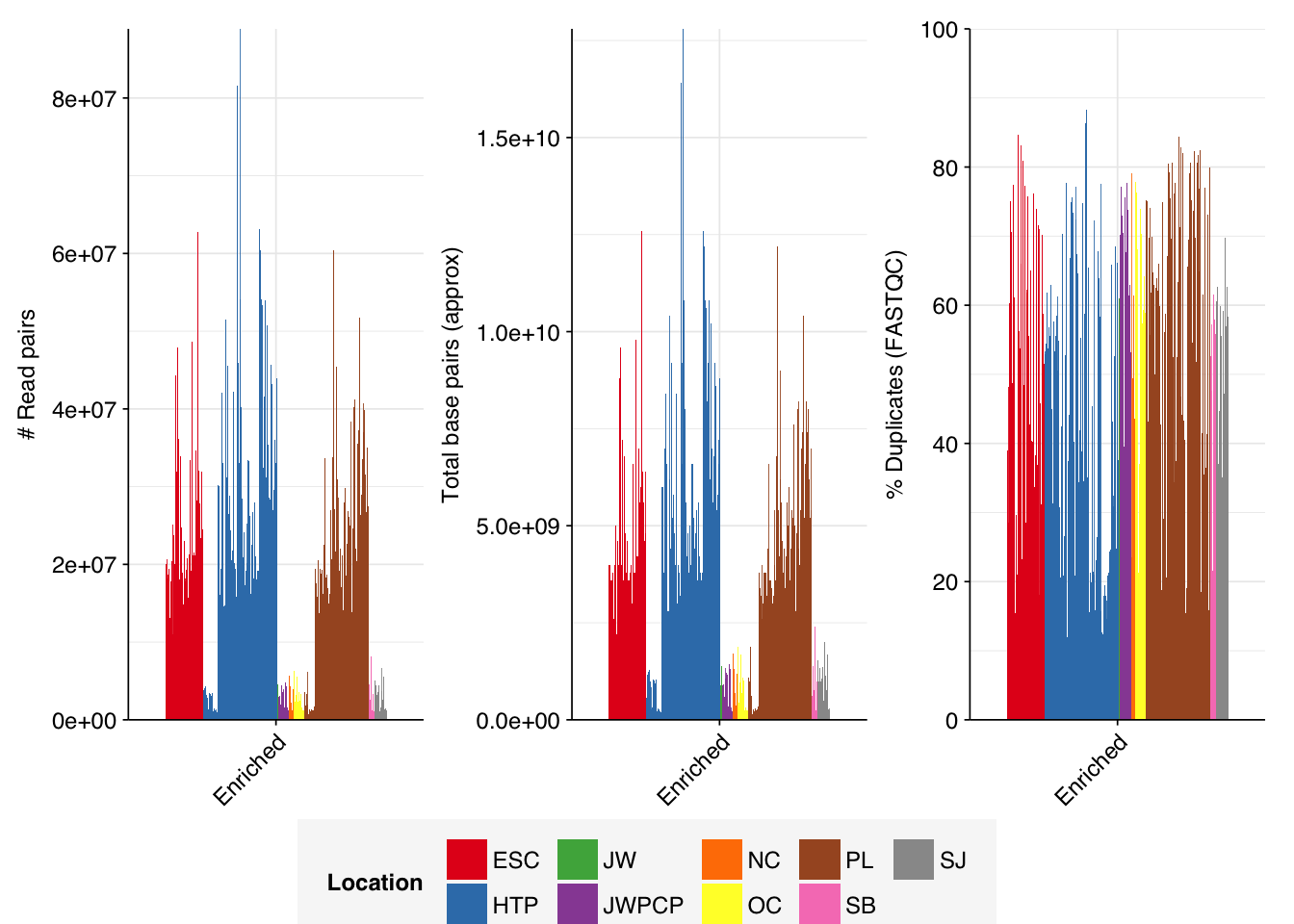
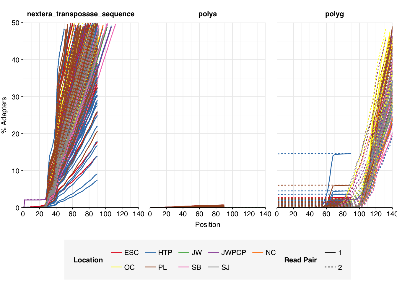
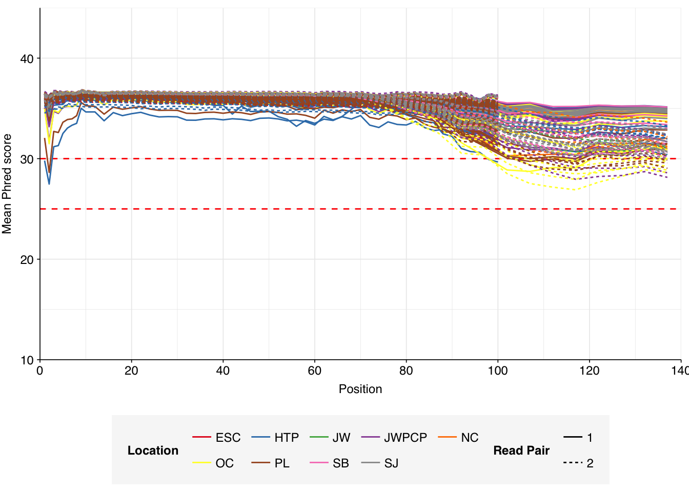
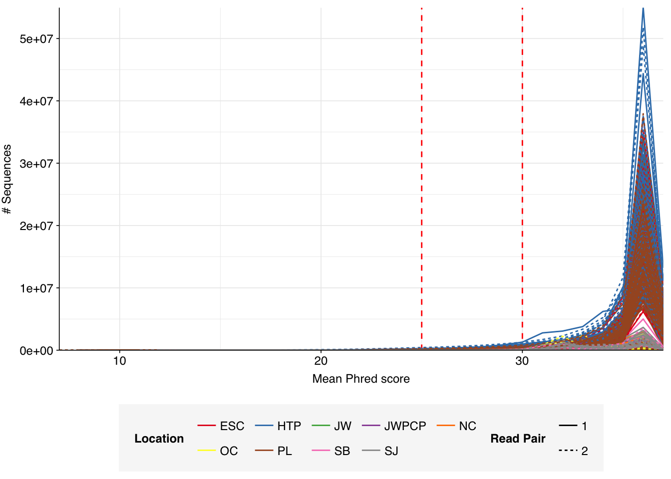
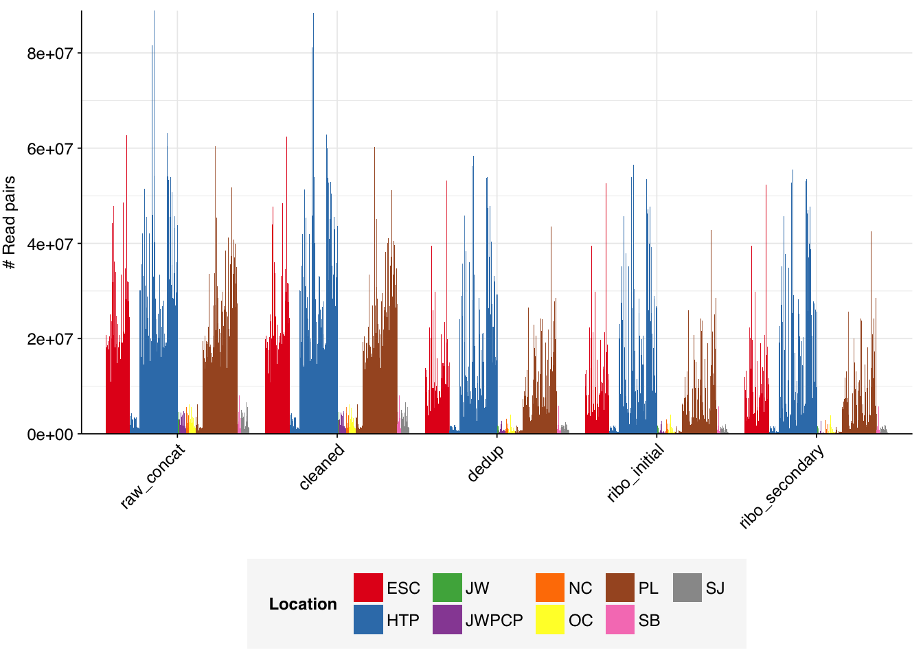
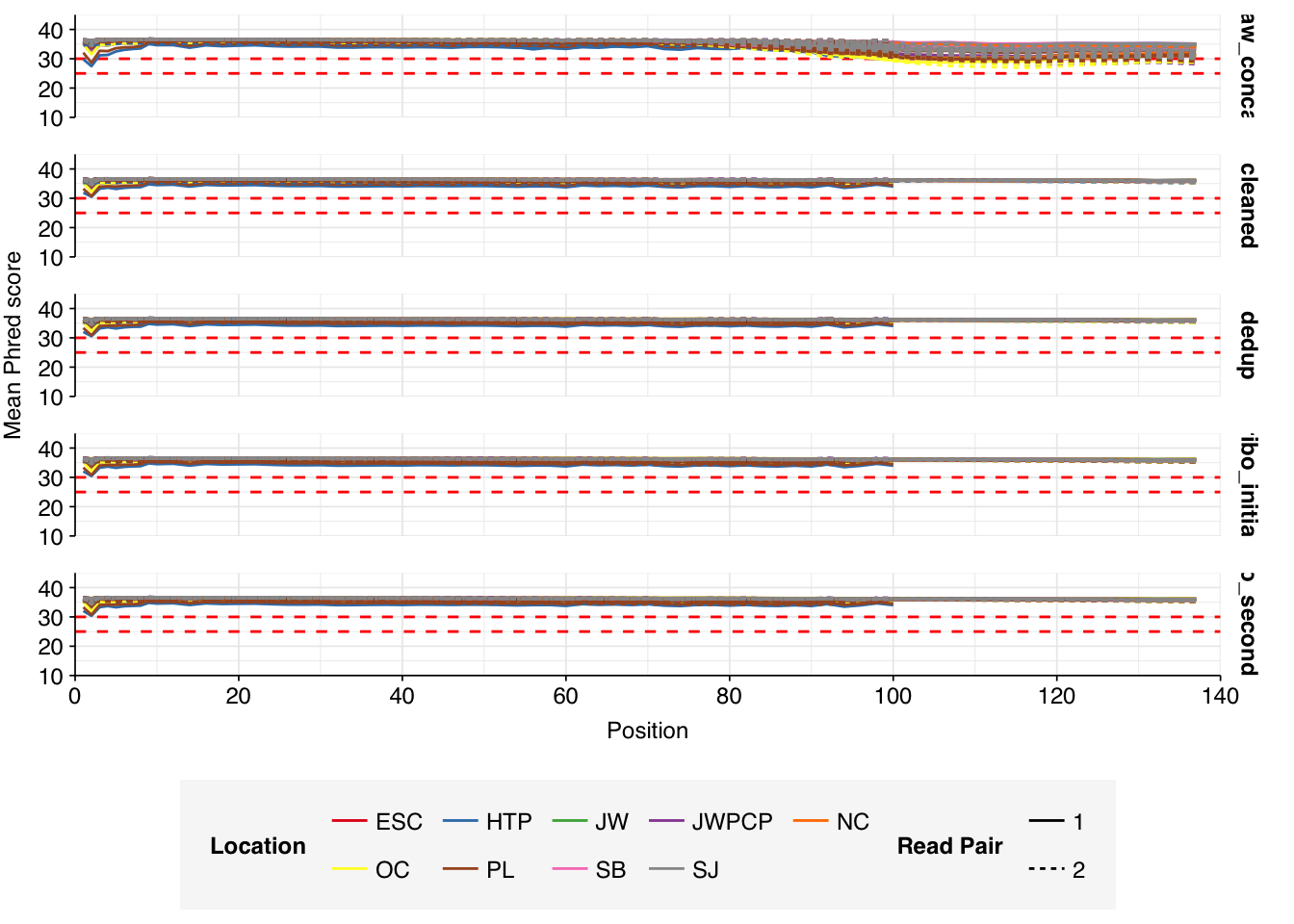
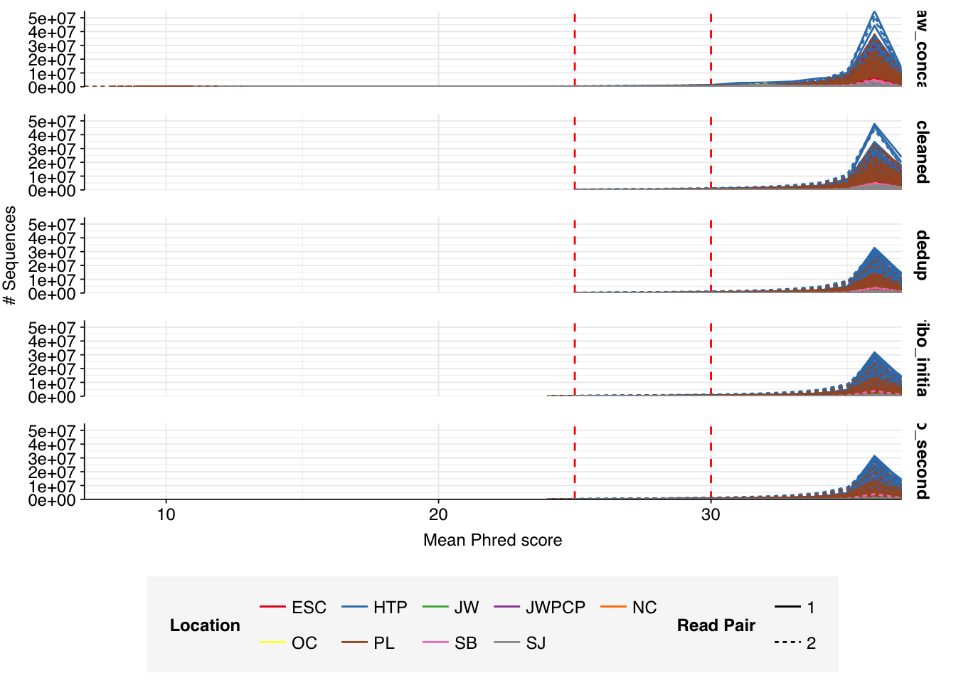
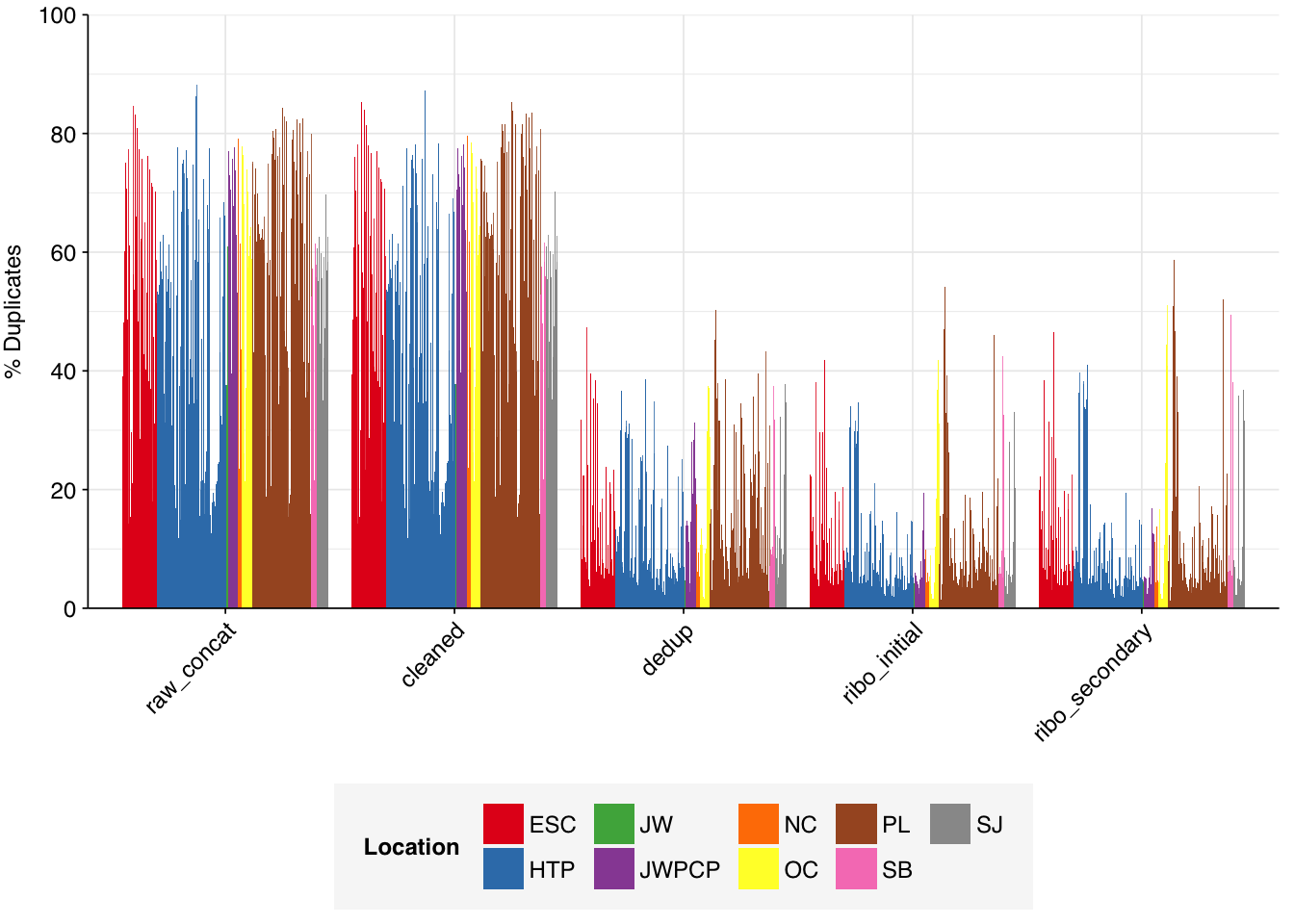
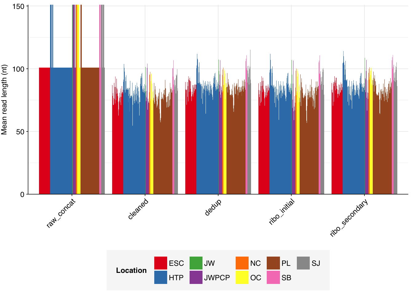
The Rothman panel-enriched samples totaled roughly 5.4B read pairs (1.1 terabases of sequence). The number of reads per sample varied from 1.3M to 23.5M, with an average of 6.8M reads per sample. The number of reads per treatment plant varied from 0.8M to 89M, with an average of 20M. The great majority of reads came from three treatment plant locations: ESC, HTP, and PL. Duplication and adapter levels were similar to the unenriched samples, which a median FASTQC-measured duplication level of 57%. Read qualities were high, albeit with a dropoff towards the end of longer reads; the large mid-read drop seen in some unenriched samples was not observed here.

Code

# Data input paths
data_dir <- "../data/2024-02-29_rothman-2"
libraries_path <- file.path(data_dir, "rothman-libraries-enriched.csv")
basic_stats_path <- file.path(data_dir, "qc_basic_stats.tsv")
adapter_stats_path <- file.path(data_dir, "qc_adapter_stats.tsv")
quality_base_stats_path <- file.path(data_dir, "qc_quality_base_stats.tsv")
quality_seq_stats_path <- file.path(data_dir, "qc_quality_sequence_stats.tsv")

# Import libraries and extract metadata from sample names
libraries <- read_csv(libraries_path, show_col_types = FALSE) %>%
  separate(sample, c("location", "month", "day", "year", "x1", "x2"), remove = FALSE) %>%
  mutate(month = as.numeric(month), year = as.numeric(year), day = as.numeric(day),
         enrichment = "Enriched", 
         date = ymd(paste(year, month, day, sep="-"))) %>%
  select(-x1, -x2) %>%
  arrange(enrichment, location, date) %>%
  mutate(location = fct_inorder(location))

# Import QC data
stages <- c("raw_concat", "cleaned", "dedup", "ribo_initial", "ribo_secondary")
basic_stats <- read_tsv(basic_stats_path, show_col_types = FALSE) %>%
  mutate(sample = sub("_2$", "", sample)) %>%
  inner_join(libraries, by="sample") %>% 
  arrange(enrichment, location, date) %>%
  mutate(stage = factor(stage, levels = stages),
         sample = fct_inorder(sample))
adapter_stats <- read_tsv(adapter_stats_path, show_col_types = FALSE) %>%
    mutate(sample = sub("_2$", "", sample)) %>%
  inner_join(libraries, by="sample") %>%
  mutate(stage = factor(stage, levels = stages),
         read_pair = fct_inorder(as.character(read_pair)))
quality_base_stats <- read_tsv(quality_base_stats_path, show_col_types = FALSE) %>%
    mutate(sample = sub("_2$", "", sample)) %>%
  inner_join(libraries, by="sample") %>%
  mutate(stage = factor(stage, levels = stages),
         read_pair = fct_inorder(as.character(read_pair)))
quality_seq_stats <- read_tsv(quality_seq_stats_path, show_col_types = FALSE) %>%
    mutate(sample = sub("_2$", "", sample)) %>%
  inner_join(libraries, by="sample") %>%
  mutate(stage = factor(stage, levels = stages),
         read_pair = fct_inorder(as.character(read_pair)))

# Filter to raw data
basic_stats_raw <- basic_stats %>% filter(stage == "raw_concat")
adapter_stats_raw <- adapter_stats %>% filter(stage == "raw_concat")
quality_base_stats_raw <- quality_base_stats %>% filter(stage == "raw_concat")
quality_seq_stats_raw <- quality_seq_stats %>% filter(stage == "raw_concat")

# Visualize basic stats
g_nreads_raw <- ggplot(basic_stats_raw, aes(x=enrichment, y=n_read_pairs, fill=location, group=sample)) + geom_col(position="dodge") + scale_y_continuous(name="# Read pairs", expand=c(0,0)) + scale_fill_brewer(palette="Set1", name="Location") + theme_kit
legend_location <- get_legend(g_nreads_raw)
g_nreads_raw_2 <- g_nreads_raw + theme(legend.position = "none")
g_nbases_raw <- ggplot(basic_stats_raw, aes(x=enrichment, y=n_bases_approx, fill=location, group=sample)) + geom_col(position="dodge") + scale_y_continuous(name="Total base pairs (approx)", expand=c(0,0)) + scale_fill_brewer(palette="Set1", name="Location") + theme_kit + theme(legend.position = "none")
g_ndup_raw <- ggplot(basic_stats_raw, aes(x=enrichment, y=percent_duplicates, fill=location, group=sample)) + geom_col(position="dodge") + scale_y_continuous(name="% Duplicates (FASTQC)", expand=c(0,0), limits = c(0,100), breaks = seq(0,100,20)) + scale_fill_brewer(palette="Set1", name="Location") + theme_kit + theme(legend.position = "none")
g_basic_raw <- plot_grid(g_nreads_raw_2 + g_nbases_raw + g_ndup_raw, legend_location, ncol = 1, rel_heights = c(1,0.1))
g_basic_raw

Code

# Visualize adapters
g_adapters_raw <- ggplot(adapter_stats_raw, aes(x=position, y=pc_adapters, color=location, linetype = read_pair, group=interaction(sample, read_pair))) + geom_line() +
  scale_color_brewer(palette = "Set1", name = "Location") +
  scale_linetype_discrete(name = "Read Pair") +
  scale_y_continuous(name="% Adapters", limits=c(0,50),
                     breaks = seq(0,50,10), expand=c(0,0)) +
  scale_x_continuous(name="Position", limits=c(0,140),
                     breaks=seq(0,140,20), expand=c(0,0)) +
  guides(color=guide_legend(nrow=2,byrow=TRUE),
         linetype = guide_legend(nrow=2,byrow=TRUE)) +
  facet_wrap(~adapter) + theme_base
g_adapters_raw

Code

# Visualize quality
g_quality_base_raw <- ggplot(quality_base_stats_raw, aes(x=position, y=mean_phred_score, color=location, linetype = read_pair, group=interaction(sample,read_pair))) +
  geom_hline(yintercept=25, linetype="dashed", color="red") +
  geom_hline(yintercept=30, linetype="dashed", color="red") +
  geom_line() +
  scale_color_brewer(palette = "Set1", name = "Location") +
  scale_linetype_discrete(name = "Read Pair") +
  scale_y_continuous(name="Mean Phred score", expand=c(0,0), limits=c(10,45)) +
  scale_x_continuous(name="Position", limits=c(0,140),
                     breaks=seq(0,140,20), expand=c(0,0)) +
  guides(color=guide_legend(nrow=2,byrow=TRUE),
         linetype = guide_legend(nrow=2,byrow=TRUE)) +
  theme_base
g_quality_seq_raw <- ggplot(quality_seq_stats_raw, aes(x=mean_phred_score, y=n_sequences, color=location, linetype = read_pair, group=interaction(sample,read_pair))) +
  geom_vline(xintercept=25, linetype="dashed", color="red") +
  geom_vline(xintercept=30, linetype="dashed", color="red") +
  geom_line() +
  scale_color_brewer(palette = "Set1", name = "Location") +
  scale_linetype_discrete(name = "Read Pair") +
  scale_x_continuous(name="Mean Phred score", expand=c(0,0)) +
  scale_y_continuous(name="# Sequences", expand=c(0,0)) +
  guides(color=guide_legend(nrow=2,byrow=TRUE),
         linetype = guide_legend(nrow=2,byrow=TRUE)) +
  theme_base
g_quality_base_raw

Code

g_quality_seq_raw

Preprocessing

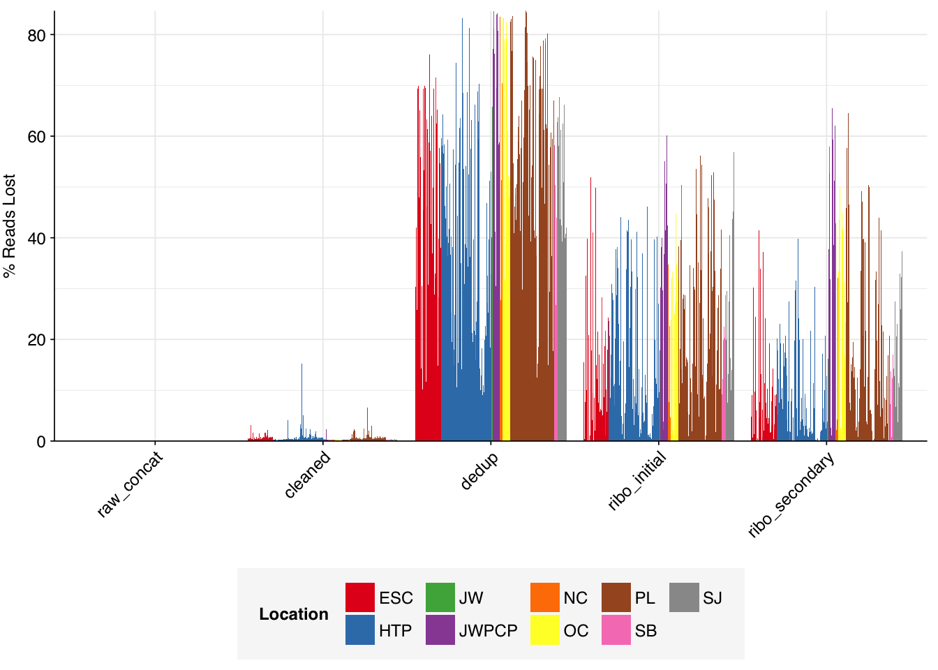
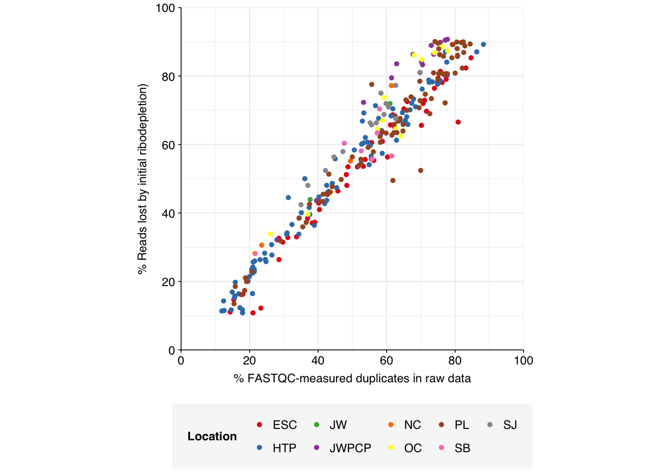
Deduplication and conservative ribodepletion together removed about 57% of total reads on average, similar to unenriched samples. Secondary ribodepletion removing a further 4% on average. However, as before, these summary figures conceal significant inter-sample variation, with samples that showed a higher initial level of duplication also showing greater read losses during preprocessing.

Code

# Plot reads over preprocessing
g_reads_stages <- ggplot(basic_stats, aes(x=stage, y=n_read_pairs,fill=location,group=sample)) +
  geom_col(position="dodge") + scale_fill_brewer(palette="Set1", name="Location") +
  scale_y_continuous("# Read pairs", expand=c(0,0)) +
  theme_kit
g_reads_stages

Code

# Plot relative read losses during preprocessing
n_reads_rel <- basic_stats %>% select(sample, location, stage, enrichment, percent_duplicates, n_read_pairs) %>%
  group_by(sample, location, enrichment) %>% arrange(sample, location, enrichment, stage) %>%
  mutate(p_reads_retained = n_read_pairs / lag(n_read_pairs),
         p_reads_lost = 1 - p_reads_retained,
         p_reads_retained_abs = n_read_pairs / n_read_pairs[1],
         p_reads_lost_abs = 1-p_reads_retained_abs)
g_reads_rel <- ggplot(n_reads_rel, aes(x=stage, y=p_reads_lost,fill=location,group=sample)) +
  geom_col(position="dodge") + scale_fill_brewer(palette="Set1", name="Location") +
  scale_y_continuous("% Reads Lost", expand=c(0,0), labels = function(x) x*100) +
  theme_kit
g_reads_rel

Code

# Plot read losses vs initial duplication levels
g_loss_dup <- n_reads_rel %>% 
  mutate(percent_duplicates_raw = percent_duplicates[1]) %>% 
  filter(stage == "ribo_initial") %>% 
  ggplot(aes(x=percent_duplicates_raw, y=p_reads_lost_abs, color=location)) + 
  geom_point(shape = 16) +
  scale_color_brewer(palette="Set1", name="Location") +
  scale_y_continuous("% Reads lost by initial ribodepletion)", expand=c(0,0), labels = function(x) x*100, breaks = seq(0,1,0.2), limits = c(0,1)) +
  scale_x_continuous("% FASTQC-measured duplicates in raw data", expand=c(0,0),
                     breaks = seq(0,100,20), limits=c(0,100)) +
  theme_base + theme(aspect.ratio = 1)
g_loss_dup

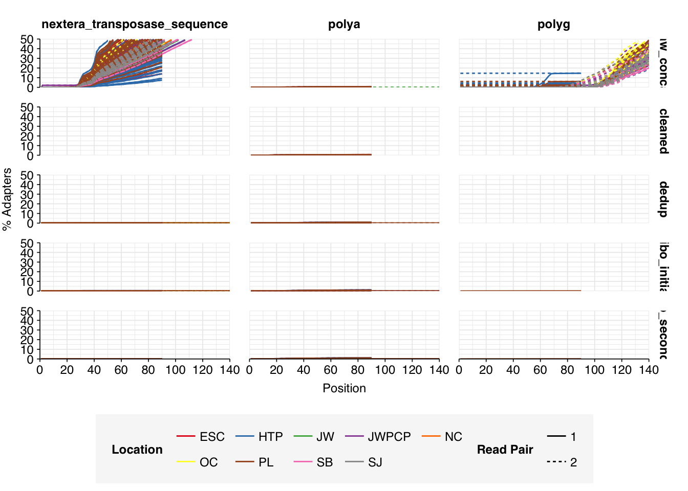
Data cleaning with FASTP was very successful at removing adapters, with no adapter sequences found by FASTQC at any stage after the raw data. Preprocessing successfully removed the terminal decline in quality seen in many samples.

Code

# Visualize adapters
g_adapters <- ggplot(adapter_stats, aes(x=position, y=pc_adapters, color=location, linetype = read_pair, group=interaction(sample, read_pair))) + geom_line() +
  scale_color_brewer(palette = "Set1", name = "Location") +
  scale_linetype_discrete(name = "Read Pair") +
  scale_y_continuous(name="% Adapters", limits=c(0,50),
                     breaks = seq(0,50,10), expand=c(0,0)) +
  scale_x_continuous(name="Position", limits=c(0,140),
                     breaks=seq(0,140,20), expand=c(0,0)) +
  guides(color=guide_legend(nrow=2,byrow=TRUE),
         linetype = guide_legend(nrow=2,byrow=TRUE)) +
  facet_grid(stage~adapter) + theme_base
g_adapters

Code

# Visualize quality
g_quality_base <- ggplot(quality_base_stats, aes(x=position, y=mean_phred_score, color=location, linetype = read_pair, group=interaction(sample,read_pair))) +
  geom_hline(yintercept=25, linetype="dashed", color="red") +
  geom_hline(yintercept=30, linetype="dashed", color="red") +
  geom_line() +
  scale_color_brewer(palette = "Set1", name = "Location") +
  scale_linetype_discrete(name = "Read Pair") +
  scale_y_continuous(name="Mean Phred score", expand=c(0,0), limits=c(10,45)) +
  scale_x_continuous(name="Position", limits=c(0,140),
                     breaks=seq(0,140,20), expand=c(0,0)) +
  guides(color=guide_legend(nrow=2,byrow=TRUE),
         linetype = guide_legend(nrow=2,byrow=TRUE)) +
  facet_grid(stage~.) + theme_base
g_quality_seq <- ggplot(quality_seq_stats, aes(x=mean_phred_score, y=n_sequences, color=location, linetype = read_pair, group=interaction(sample,read_pair))) +
  geom_vline(xintercept=25, linetype="dashed", color="red") +
  geom_vline(xintercept=30, linetype="dashed", color="red") +
  geom_line() +
  scale_color_brewer(palette = "Set1", name = "Location") +
  scale_linetype_discrete(name = "Read Pair") +
  scale_x_continuous(name="Mean Phred score", expand=c(0,0)) +
  scale_y_continuous(name="# Sequences", expand=c(0,0)) +
  guides(color=guide_legend(nrow=2,byrow=TRUE),
         linetype = guide_legend(nrow=2,byrow=TRUE)) +
  facet_grid(stage~.) + theme_base
g_quality_base

Code

g_quality_seq

Deduplication and ribodepletion were collectively quite effective at reducing measured duplicate levels, with the average detected duplication level after both processes reduced to roughly 11%. Note that the pipeline still doesn’t have a reverse-complement-sensitive deduplication pipeline, so only same-orientation duplicates have been removed.

Code

g_dup_stages <- ggplot(basic_stats, aes(x=stage, y=percent_duplicates, fill=location, group=sample)) +
  geom_col(position="dodge") + scale_fill_brewer(palette = "Set1", name="Location") +
  scale_y_continuous("% Duplicates", limits=c(0,100), breaks=seq(0,100,20), expand=c(0,0)) +
  theme_kit
g_readlen_stages <- ggplot(basic_stats, aes(x=stage, y=mean_seq_len, fill=location, group=sample)) +
  geom_col(position="dodge") + scale_fill_brewer(palette = "Set1", name="Location") +
  scale_y_continuous("Mean read length (nt)", expand=c(0,0)) +
  theme_kit
legend_loc <- get_legend(g_dup_stages)
g_dup_stages

Code

g_readlen_stages

High-level composition

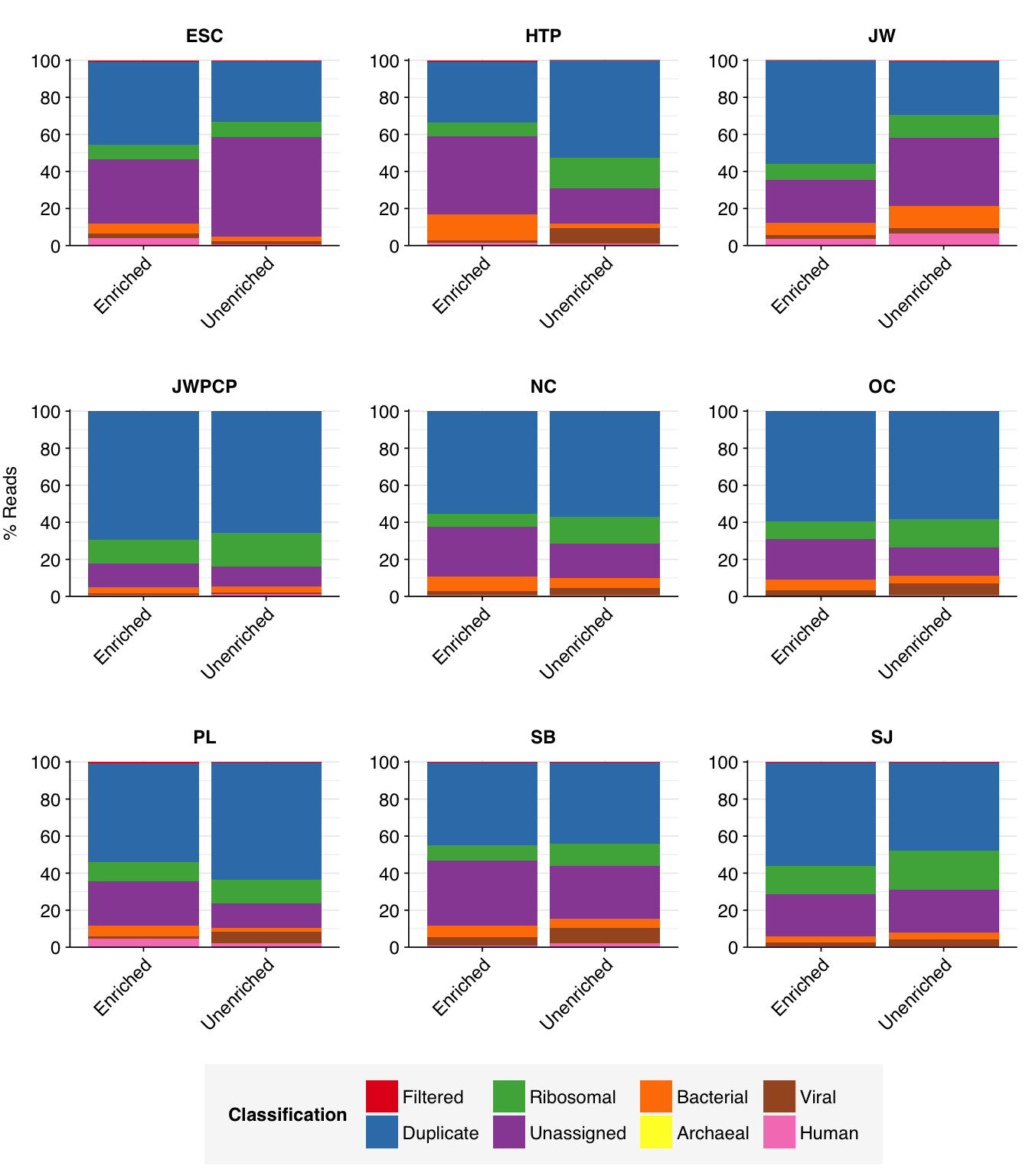
As before, to assess the high-level composition of the reads, I ran the ribodepleted files through Kraken (using the Standard 16 database) and summarized the results with Bracken. Combining these results with the read counts above gives us a breakdown of the inferred composition of the samples:

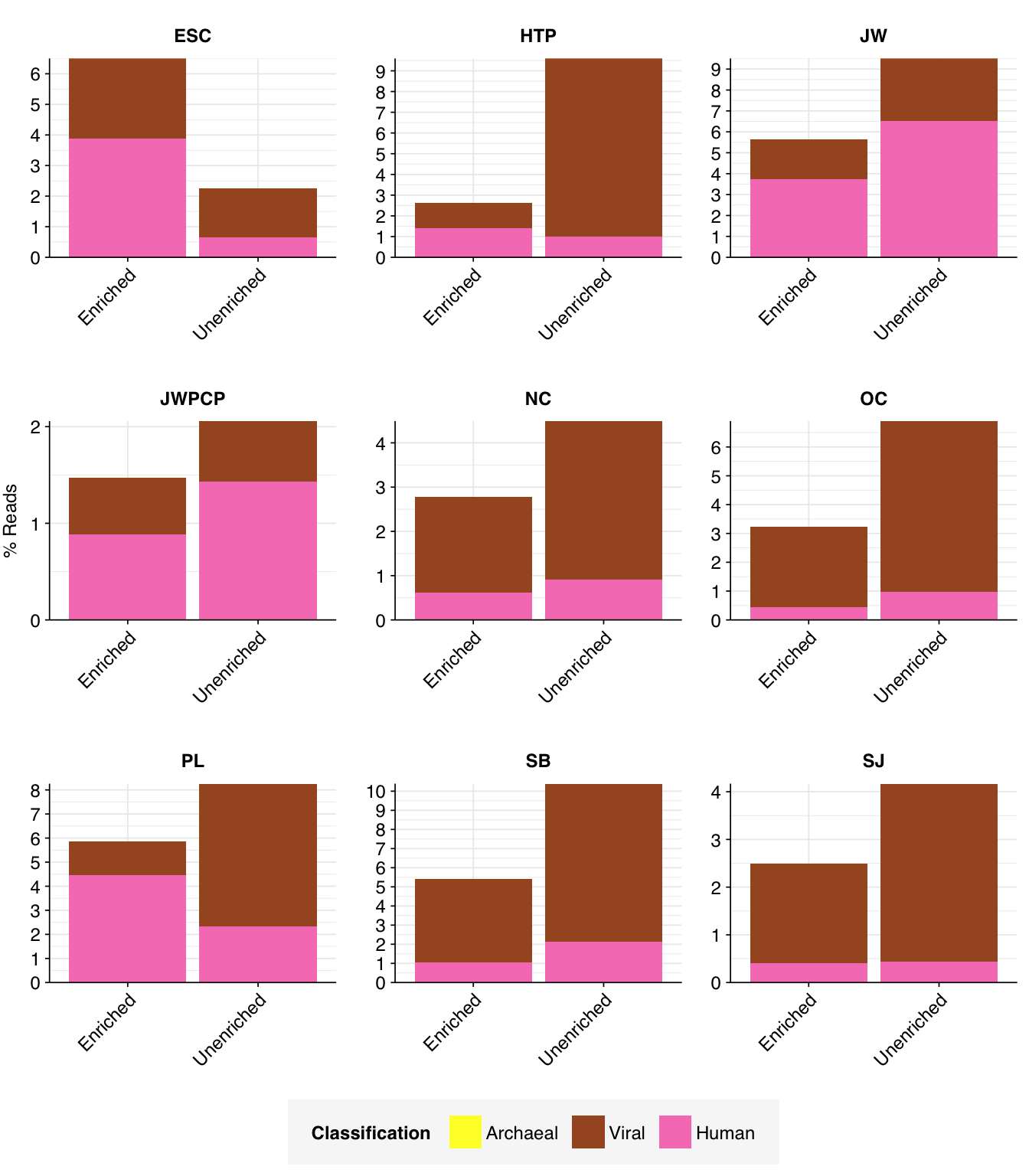
Code

# Import data for unenriched samples
data_dir_old <- "../data/2024-02-23_rothman-1/"
bracken_path_old <- file.path(data_dir_old, "bracken_counts.tsv")
basic_stats_path_old <- file.path(data_dir_old, "qc_basic_stats.tsv")
libraries_path_old <- file.path(data_dir_old, "rothman-libraries-unenriched.csv")

bracken_old <- read_tsv(bracken_path_old, show_col_types = FALSE)
libraries_old <- read_csv(libraries_path_old, show_col_types = FALSE) %>%
  separate(sample, c("location", "month", "day", "year", "x1", "x2"), remove = FALSE) %>%
  mutate(month = as.numeric(month), year = as.numeric(year), day = as.numeric(day),
         enrichment = "Unenriched", 
         date = ymd(paste(year, month, day, sep="-"))) %>%
  select(-x1, -x2) %>%
  arrange(enrichment, location, date) %>%
  mutate(location = fct_inorder(location))
basic_stats_old <- read_tsv(basic_stats_path_old, show_col_types = FALSE) %>%
  mutate(sample = sub("_2$", "", sample)) %>%
  inner_join(libraries_old, by="sample") %>% 
  arrange(enrichment, location, date) %>%
  mutate(stage = factor(stage, levels = stages),
         sample = fct_inorder(sample))

# Import Bracken data
bracken_path <- file.path(data_dir, "bracken_counts.tsv")
bracken <- read_tsv(bracken_path, show_col_types = FALSE)
total_assigned <- bracken %>% group_by(sample) %>% summarize(
  name = "Total",
  kraken_assigned_reads = sum(kraken_assigned_reads),
  added_reads = sum(added_reads),
  new_est_reads = sum(new_est_reads),
  fraction_total_reads = sum(fraction_total_reads)
)
bracken_spread <- bracken %>% select(name, sample, new_est_reads) %>%
  mutate(name = tolower(name)) %>%
  pivot_wider(id_cols = "sample", names_from = "name", values_from = "new_est_reads")
total_assigned_old <- bracken_old %>% group_by(sample) %>% summarize(
  name = "Total",
  kraken_assigned_reads = sum(kraken_assigned_reads),
  added_reads = sum(added_reads),
  new_est_reads = sum(new_est_reads),
  fraction_total_reads = sum(fraction_total_reads)
)
bracken_spread_old <- bracken_old %>% select(name, sample, new_est_reads) %>%
  mutate(name = tolower(name)) %>%
  pivot_wider(id_cols = "sample", names_from = "name", values_from = "new_est_reads")

# Count reads
read_counts_preproc <- basic_stats %>% 
  select(sample, location, enrichment, stage, n_read_pairs) %>%
  pivot_wider(id_cols = c("sample", "location", "enrichment"), names_from="stage", values_from="n_read_pairs")
read_counts <- read_counts_preproc %>%
  inner_join(total_assigned %>% select(sample, new_est_reads), by = "sample") %>%
  rename(assigned = new_est_reads) %>%
  inner_join(bracken_spread, by="sample")
read_counts_preproc_old <- basic_stats_old %>% 
  select(sample, location, enrichment, stage, n_read_pairs) %>%
  pivot_wider(id_cols = c("sample", "location", "enrichment"), names_from="stage", values_from="n_read_pairs")
read_counts_old <- read_counts_preproc_old %>%
  inner_join(total_assigned_old %>% select(sample, new_est_reads), by = "sample") %>%
  rename(assigned = new_est_reads) %>%
  inner_join(bracken_spread_old, by="sample")

# Assess composition
read_comp <- transmute(read_counts, sample=sample, location=location,
                       enrichment=enrichment,
                       n_filtered = raw_concat-cleaned,
                       n_duplicate = cleaned-dedup,
                       n_ribosomal = (dedup-ribo_initial) + (ribo_initial-ribo_secondary),
                       n_unassigned = ribo_secondary-assigned,
                       n_bacterial = bacteria,
                       n_archaeal = archaea,
                       n_viral = viruses,
                       n_human = eukaryota)
read_comp_long <- pivot_longer(read_comp, -(sample:enrichment), names_to = "classification",
                               names_prefix = "n_", values_to = "n_reads") %>%
  mutate(classification = fct_inorder(str_to_sentence(classification))) %>%
  group_by(sample) %>% mutate(p_reads = n_reads/sum(n_reads))
read_comp_summ <- read_comp_long %>% 
  group_by(location, enrichment, classification) %>%
  summarize(n_reads = sum(n_reads), .groups = "drop_last") %>%
  mutate(n_reads = replace_na(n_reads,0),
    p_reads = n_reads/sum(n_reads),
    pc_reads = p_reads*100)
read_comp_old <- transmute(read_counts_old, sample=sample, location=location,
                       enrichment=enrichment,
                       n_filtered = raw_concat-cleaned,
                       n_duplicate = cleaned-dedup,
                       n_ribosomal = (dedup-ribo_initial) + (ribo_initial-ribo_secondary),
                       n_unassigned = ribo_secondary-assigned,
                       n_bacterial = bacteria,
                       n_archaeal = archaea,
                       n_viral = viruses,
                       n_human = eukaryota)
read_comp_long_old <- pivot_longer(read_comp_old, -(sample:enrichment), 
                                   names_to = "classification",
                                   names_prefix = "n_", values_to = "n_reads") %>%
  mutate(classification = fct_inorder(str_to_sentence(classification))) %>%
  group_by(sample) %>% mutate(p_reads = n_reads/sum(n_reads))
read_comp_summ_old <- read_comp_long_old %>% 
  group_by(location, enrichment, classification) %>%
  summarize(n_reads = sum(n_reads), .groups = "drop_last") %>%
  mutate(n_reads = replace_na(n_reads,0),
    p_reads = n_reads/sum(n_reads),
    pc_reads = p_reads*100)

# Merge data
read_comp_mrg <- bind_rows(read_comp_summ %>% mutate(enrichment = "Enriched"),
                           read_comp_summ_old %>% mutate(enrichment = "Unenriched"))
  
# Plot overall composition
g_comp <- ggplot(read_comp_mrg, aes(x=enrichment, y=p_reads, fill=classification)) +
  geom_col(position = "stack") +
  scale_y_continuous(name = "% Reads", limits = c(0,1.01), breaks = seq(0,1,0.2),
                     expand = c(0,0), labels = function(x) x*100) +
  scale_fill_brewer(palette = "Set1", name = "Classification") +
  facet_wrap(.~location, scales="free") +
  theme_kit
g_comp

Code

# Plot composition of minor components
read_comp_minor <- read_comp_mrg %>% filter(classification %in% c("Archaeal", "Viral", "Human", "Other"))
palette_minor <- brewer.pal(9, "Set1")[6:9]
g_comp_minor <- ggplot(read_comp_minor, aes(x=enrichment, y=p_reads, fill=classification)) +
  geom_col(position = "stack") +
  scale_y_continuous(name = "% Reads", breaks = seq(0,0.1,0.01),
                     expand = c(0,0), labels = function(x) x*100) +
  scale_fill_manual(values=palette_minor, name = "Classification") +
  facet_wrap(.~location, scales="free") +
  theme_kit
g_comp_minor

The average fraction of low-quality, duplicate, and unassigned reads is slightly higher in enriched vs unenriched samples (mean 80% vs 75%), while the average fraction of ribosomal reads is lower (10% vs 15%). The fraction of bacterial reads is similar (7% vs 5%), while the overall fraction of viral reads is actually slightly lower (2% vs 5%). This latter finding is perhaps surprising, given that the enriched samples are enriched for a group of viruses; I suspect the observed results are due to non-human viruses (especially tobamoviruses) dominating human viruses in the overall counts.

Human-infecting virus reads

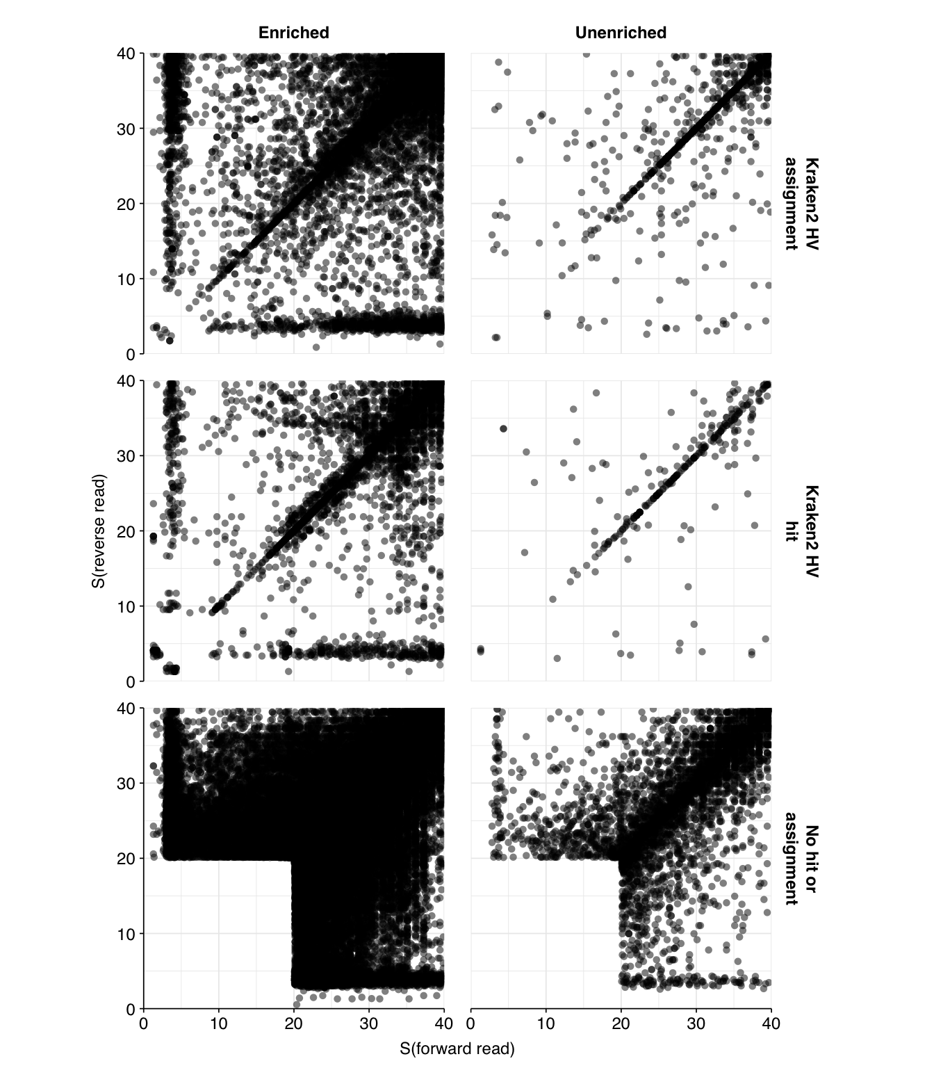
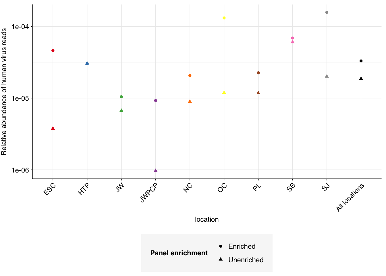
Now we come to the main result of interest: the fraction of human-infecting virus reads in enriched vs unenriched samples.

Code

# New HV reads
hv_reads_filtered_path <- file.path(data_dir, "hv_hits_putative_filtered.tsv.gz")
hv_reads_filtered <- read_tsv(hv_reads_filtered_path, show_col_types = FALSE) %>%
  inner_join(libraries, by="sample") %>% 
  arrange(enrichment, location, date) %>%
  mutate(sample = fct_inorder(sample))

# Old HV reads
hv_reads_filtered_path_old <- file.path(data_dir_old, "hv_hits_putative_filtered.tsv.gz")
hv_reads_filtered_old <- read_tsv(hv_reads_filtered_path_old, show_col_types = FALSE) %>%
  inner_join(libraries_old, by="sample") %>% 
  arrange(enrichment, location, date) %>%
  mutate(sample = fct_inorder(sample))

# Combined
mrg <- bind_rows(hv_reads_filtered, hv_reads_filtered_old) %>%
  mutate(kraken_label = ifelse(assigned_hv, "Kraken2 HV\nassignment",
                               ifelse(hit_hv, "Kraken2 HV\nhit",
                                      "No hit or\nassignment"))) %>%
  group_by(sample) %>% arrange(desc(adj_score_fwd), desc(adj_score_rev)) %>%
  mutate(seq_num = row_number(),
         adj_score_max = pmax(adj_score_fwd, adj_score_rev)) %>%
  filter(assigned_hv | hit_hv | adj_score_max >= 20)
# Import Bowtie2/Kraken data and perform filtering steps
g_mrg <- ggplot(mrg, aes(x=adj_score_fwd, y=adj_score_rev)) +
  geom_point(alpha=0.5, shape=16) + 
  scale_x_continuous(name="S(forward read)", limits=c(0,40), breaks=seq(0,100,10), expand = c(0,0)) +
  scale_y_continuous(name="S(reverse read)", limits=c(0,40), breaks=seq(0,100,10), expand = c(0,0)) +
  facet_grid(kraken_label~enrichment, labeller = labeller(kit = label_wrap_gen(20))) +
  theme_base + theme(aspect.ratio=1)
g_mrg

Following the same selection criteria used for the unenriched samples, we identify 177,246 HV reads across the panel-enriched samples, compared to 12,305 in the unenriched samples. This corresponds to an overall relative HV abundance estimate of \(3.3 \times 10^{-5}\) - about double the estimate for unenriched samples of \(1.87 \times 10^{-5}\). This is much lower than the HV relative abundance observed in Crits-Christoph’s enriched samples, which exceeded \(10^{-2}\).

Panel-enriched relative abundance for individual treatment plants varied from \(9.3 \times 10^{-6}\) to \(1.6 \times 10^{-4}\), with enrichment factors compared to unenriched samples from the same plant ranging from \(1\times\) (HTP) to \(12\times\) (ESC). Overall, this seems like a relatively disappointing showing for panel-enrichment compared to some other datasets we’ve seen.

Code

# Get raw read counts
read_counts_raw <- basic_stats %>% filter(stage == "raw_concat") %>% 
  select(sample, location, enrichment, date, n_reads_raw = n_read_pairs)
read_counts_raw_old <- basic_stats_old %>% filter(stage == "raw_concat") %>% 
  select(sample, location, enrichment, date, n_reads_raw = n_read_pairs)
read_counts_raw_mrg <- bind_rows(read_counts_raw, read_counts_raw_old)

# Get HV read counts & RA
read_counts_hv_mrg <- mrg %>% group_by(sample, location, enrichment) %>%
  count(name = "n_reads_hv")
read_counts <- read_counts_raw_mrg %>%
  left_join(read_counts_hv_mrg, by=c("sample", "location", "enrichment")) %>%
  mutate(n_reads_hv = replace_na(n_reads_hv, 0),
         p_reads_hv = n_reads_hv/n_reads_raw)

# Aggregate by location
read_counts_loc <- read_counts %>% group_by(location, enrichment) %>%
  summarize(n_reads_raw = sum(n_reads_raw),
            n_reads_hv = sum(n_reads_hv), .groups = "drop") %>%
  mutate(p_reads_hv = n_reads_hv/n_reads_raw)
read_counts_total <- read_counts_loc %>% group_by(enrichment) %>%
  summarize(n_reads_raw = sum(n_reads_raw),
            n_reads_hv = sum(n_reads_hv)) %>%
  mutate(p_reads_hv = n_reads_hv/n_reads_raw,
         location = "All locations")
read_counts_agg <- read_counts_loc %>% mutate(location = as.character(location)) %>%
  bind_rows(read_counts_total) %>%
  mutate(location = fct_inorder(location))

# Calculate enrichment factors
read_counts_enrichment <- read_counts_agg %>% select(location, enrichment, p_reads_hv) %>%
  pivot_wider(id_cols = "location", names_from = enrichment, values_from = p_reads_hv) %>%
  mutate(enrichment = Enriched/Unenriched)

# Visualize
palette_loc <- c(brewer.pal(9, "Set1"), "black")
g_phv_agg <- ggplot(read_counts_agg, aes(x=location, y=p_reads_hv, color=location, 
                                         shape=enrichment)) +
  geom_point() +
  scale_y_log10("Relative abundance of human virus reads") +
  scale_color_manual(values=palette_loc, name="Location") +
  scale_shape_discrete(name = "Panel enrichment") +
  guides(shape = guide_legend(nrow=2, vjust=0.5), color="none") +
  theme_base + theme(axis.text.x = element_text(angle=45, hjust=1))
g_phv_agg

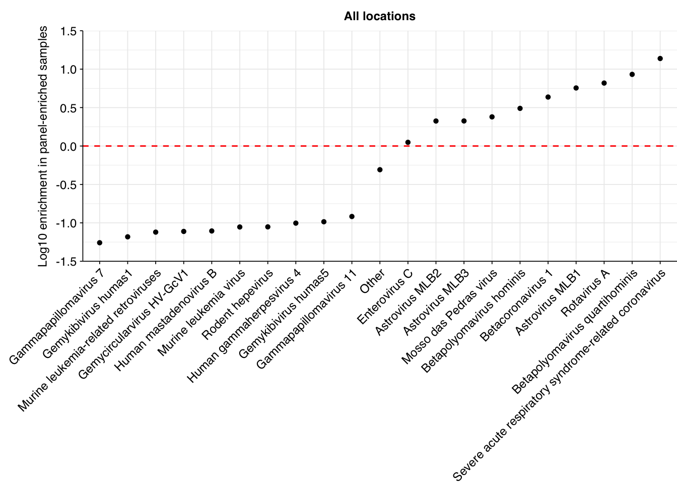
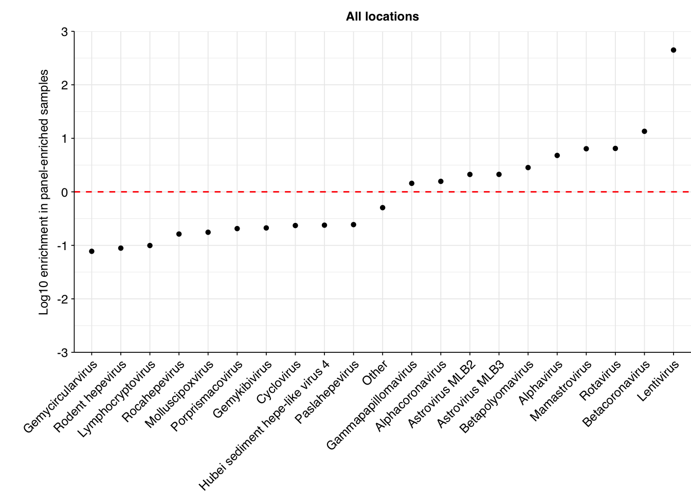
Digging into specific viruses, the results are…odd. While the list of most highly enriched viruses encludes some included in the Illumina panel (e.g. SARS-CoVs, betapolyomaviruses), many are fecal-oral viruses with no obvious relationship to the panel (e.g. various astroviruses). The most highly enriched viral genus is Lentivirus, which includes HIV and is not included in the Illumina panel. I don’t know enough about the panel or these respective viruses to give a strong take on what’s going on here, but it certainly seems that the Illumina RVP is less effective at enriching for specific respiratory viruses in Rothman than in Crits-Christoph.

Code

viral_taxa_path <- file.path(data_dir_old, "viral-taxa.tsv.gz")
viral_taxa <- read_tsv(viral_taxa_path, show_col_types = FALSE)

# Get viral taxon names for putative HV reads
mrg_named <- mrg %>% left_join(viral_taxa, by="taxid")

# Discover viral species & genera for HV reads
raise_rank <- function(read_db, taxid_db, out_rank = "species", verbose = FALSE){
  # Get higher ranks than search rank
  ranks <- c("subspecies", "species", "subgenus", "genus", "subfamily", "family", "suborder", "order", "class", "subphylum", "phylum", "kingdom", "superkingdom")
  rank_match <- which.max(ranks == out_rank)
  high_ranks <- ranks[rank_match:length(ranks)]
  # Merge read DB and taxid DB
  reads <- read_db %>% select(-parent_taxid, -rank, -name) %>%
    left_join(taxid_db, by="taxid")
  # Extract sequences that are already at appropriate rank
  reads_rank <- filter(reads, rank == out_rank)
  # Drop sequences at a higher rank and return unclassified sequences
  reads_norank <- reads %>% filter(rank != out_rank, !rank %in% high_ranks, !is.na(taxid))
  while(nrow(reads_norank) > 0){ # As long as there are unclassified sequences...
    # Promote read taxids and re-merge with taxid DB, then re-classify and filter
    reads_remaining <- reads_norank %>% mutate(taxid = parent_taxid) %>%
      select(-parent_taxid, -rank, -name) %>%
      left_join(taxid_db, by="taxid")
    reads_rank <- reads_remaining %>% filter(rank == out_rank) %>%
      bind_rows(reads_rank)
    reads_norank <- reads_remaining %>%
      filter(rank != out_rank, !rank %in% high_ranks, !is.na(taxid))
  }
  # Finally, extract and append reads that were excluded during the process
  reads_dropped <- reads %>% filter(!seq_id %in% reads_rank$seq_id)
  reads_out <- reads_rank %>% bind_rows(reads_dropped) %>%
    select(-parent_taxid, -rank, -name) %>%
    left_join(taxid_db, by="taxid")
  return(reads_out)
}

hv_reads_species <- raise_rank(mrg_named, viral_taxa, "species")
hv_reads_genera <- raise_rank(mrg_named, viral_taxa, "genus")

# Count relative abundance for species
hv_species_counts_raw <- hv_reads_species %>% group_by(location, enrichment, name) %>%
  count(name="n_reads_hv") %>%
  inner_join(read_counts_agg %>% select(location, enrichment, n_reads_raw), 
             by=c("location", "enrichment"))
hv_species_counts_all <- hv_species_counts_raw %>% group_by(name, enrichment) %>%
  summarize(n_reads_hv = sum(n_reads_hv),
            n_reads_raw = sum(n_reads_raw), .groups = "drop") %>%
  mutate(location = "All locations")
hv_species_counts_agg <- bind_rows(hv_species_counts_raw, hv_species_counts_all) %>%
  mutate(p_reads_hv = n_reads_hv/n_reads_raw)

# Count relative abundance for genera
hv_genera_counts_raw <- hv_reads_genera %>% group_by(location, enrichment, name) %>%
  count(name="n_reads_hv") %>%
  inner_join(read_counts_agg %>% select(location, enrichment, n_reads_raw), 
             by=c("location", "enrichment"))
hv_genera_counts_all <- hv_genera_counts_raw %>% group_by(name, enrichment) %>%
  summarize(n_reads_hv = sum(n_reads_hv),
            n_reads_raw = sum(n_reads_raw), .groups = "drop") %>%
  mutate(location = "All locations")
hv_genera_counts_agg <- bind_rows(hv_genera_counts_raw, hv_genera_counts_all) %>%
  mutate(p_reads_hv = n_reads_hv/n_reads_raw)

Code

max_rank_species <- 10

# Compute species enrichment
hv_species_enr <- hv_species_counts_agg %>% filter(location == "All locations") %>%
  select(location, enrichment, name, n_reads_raw, p_reads_hv) %>%
  pivot_wider(id_cols = c("location", "name"), names_from = "enrichment", 
              values_from = c("p_reads_hv", "n_reads_raw")) %>%
  mutate(p_reads_hv_Enriched = replace_na(p_reads_hv_Enriched, 0),
         p_reads_hv_Unenriched = replace_na(p_reads_hv_Unenriched, 0),
         log_enrichment = log10(p_reads_hv_Enriched/p_reads_hv_Unenriched)) %>%
  group_by(location) %>%
  mutate(n_reads_raw_Enriched = max(n_reads_raw_Enriched, na.rm = TRUE),
         n_reads_raw_Unenriched = max(n_reads_raw_Unenriched, na.rm = TRUE))

# Identify most enriched/de-enriched species
hv_species_enr_ranked <- hv_species_enr %>% group_by(location) %>%
  filter(log_enrichment < Inf, log_enrichment > -Inf) %>%
  mutate(rank_enrichment_neg = row_number(log_enrichment),
         rank_enrichment_pos = row_number(desc(log_enrichment)),
         major = rank_enrichment_neg <= max_rank_species | rank_enrichment_pos <= max_rank_species)

# Aggregate and visualize
hv_species_enr_plot <- hv_species_enr_ranked %>%
  mutate(name_display = ifelse(major, name, "Other")) %>%
  group_by(location, name_display, n_reads_raw_Unenriched, n_reads_raw_Enriched) %>%
  summarize(n_reads_hv_Enriched = sum(p_reads_hv_Enriched * n_reads_raw_Enriched),
            n_reads_hv_Unenriched = sum(p_reads_hv_Unenriched * n_reads_raw_Unenriched),
            .groups = "drop") %>%
  mutate(p_reads_hv_Enriched = n_reads_hv_Enriched / n_reads_raw_Enriched,
         p_reads_hv_Unenriched = n_reads_hv_Unenriched / n_reads_raw_Unenriched,
         log_enrichment = log10(p_reads_hv_Enriched/p_reads_hv_Unenriched)) %>%
  arrange(log_enrichment) %>% mutate(name_display = fct_inorder(name_display))
g_species_enr <- ggplot(hv_species_enr_plot,
                       aes(x=name_display, y=log_enrichment)) +
  geom_hline(yintercept = 0, color="red", linetype = "dashed") +
  geom_point(shape=16) +
  scale_y_continuous(name = "Log10 enrichment in panel-enriched samples",
                     limits = c(-1.5,1.5), expand=c(0,0)) +
  facet_wrap(location~., scales="free", ncol=1) +
  theme_kit + theme(plot.margin = margin(l=1, unit="cm"))
g_species_enr

Code

# Single-sample viruses
hv_species_enr_solo <- hv_species_enr %>%
  filter(log_enrichment == Inf) %>%
  arrange(desc(p_reads_hv_Enriched))

Code

max_rank_genera <- 10

# Compute genus enrichment
hv_genera_enr <- hv_genera_counts_agg %>% filter(location == "All locations") %>%
  select(location, enrichment, name, n_reads_raw, p_reads_hv) %>%
  pivot_wider(id_cols = c("location", "name"), names_from = "enrichment", 
              values_from = c("p_reads_hv", "n_reads_raw")) %>%
  mutate(p_reads_hv_Enriched = replace_na(p_reads_hv_Enriched, 0),
         p_reads_hv_Unenriched = replace_na(p_reads_hv_Unenriched, 0),
         log_enrichment = log10(p_reads_hv_Enriched/p_reads_hv_Unenriched)) %>%
  group_by(location) %>%
  mutate(n_reads_raw_Enriched = max(n_reads_raw_Enriched, na.rm = TRUE),
         n_reads_raw_Unenriched = max(n_reads_raw_Unenriched, na.rm = TRUE))

# Identify most enriched/de-enriched genera
hv_genera_enr_ranked <- hv_genera_enr %>% group_by(location) %>%
  filter(log_enrichment < Inf, log_enrichment > -Inf) %>%
  mutate(rank_enrichment_neg = row_number(log_enrichment),
         rank_enrichment_pos = row_number(desc(log_enrichment)),
         major = rank_enrichment_neg <= max_rank_genera | rank_enrichment_pos <= max_rank_genera)

# Aggregate and visualize
hv_genera_enr_plot <- hv_genera_enr_ranked %>%
  mutate(name_display = ifelse(major, name, "Other")) %>%
  group_by(location, name_display, n_reads_raw_Unenriched, n_reads_raw_Enriched) %>%
  summarize(n_reads_hv_Enriched = sum(p_reads_hv_Enriched * n_reads_raw_Enriched),
            n_reads_hv_Unenriched = sum(p_reads_hv_Unenriched * n_reads_raw_Unenriched),
            .groups = "drop") %>%
  mutate(p_reads_hv_Enriched = n_reads_hv_Enriched / n_reads_raw_Enriched,
         p_reads_hv_Unenriched = n_reads_hv_Unenriched / n_reads_raw_Unenriched,
         log_enrichment = log10(p_reads_hv_Enriched/p_reads_hv_Unenriched)) %>%
  arrange(log_enrichment) %>% mutate(name_display = fct_inorder(name_display))
g_genera_enr <- ggplot(hv_genera_enr_plot,
                       aes(x=name_display, y=log_enrichment)) +
  geom_hline(yintercept = 0, color="red", linetype = "dashed") +
  geom_point(shape=16) +
  scale_y_continuous(name = "Log10 enrichment in panel-enriched samples",
                     limits = c(-3,3), expand=c(0,0)) +
  facet_wrap(location~., scales="free", ncol=1) +
  theme_kit + theme(plot.margin = margin(l=1, unit="cm"))
g_genera_enr

Code

# Single-sample viruses
hv_genera_enr_solo <- hv_genera_enr %>%
  filter(log_enrichment == Inf) %>%
  arrange(desc(p_reads_hv_Enriched))