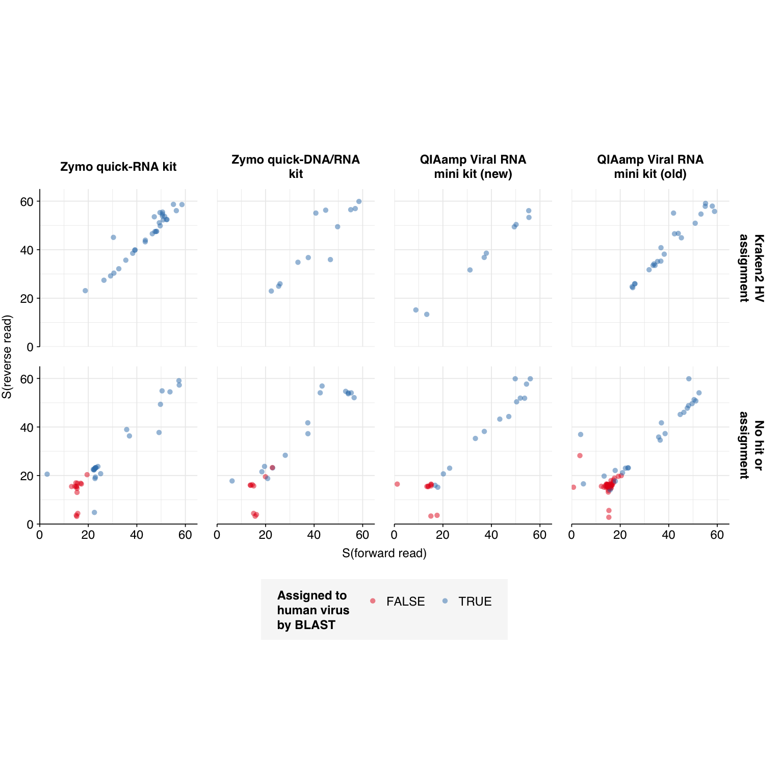
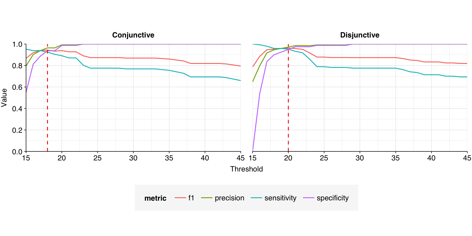
--- title: "Project Runway RNA-seq testing data: removing livestock reads" subtitle: "" author: "Will Bradshaw" date: 2023-12-22 format: html: code-fold: true code-tools: true code-link: true df-print: paged editor: visual title-block-banner: black --- ```{r} #| label: load-packages #| include: false library (tidyverse)library (cowplot)library (patchwork)library (fastqcr)source ("../scripts/aux_plot-theme.R" )<- theme_base + theme (aspect.ratio = 1 ,axis.text.x = element_text (hjust = 1 , angle = 45 ),axis.title.x = element_blank ()``` [ last entry ](https://data.securebio.org/wills-public-notebook/notebooks/2023-12-19_project-runway-bmc-rna.html) , I presented my [ Nextflow workflow ](https://github.com/naobservatory/mgs-workflow) for analyzing viral MGS data, as well as the results of that workflow applied to our recent BMC RNA-seq dataset. One surprising thing I observed in those data was the presence of bovine and porcine sequences confounding my pipeline for identifying human-infecting-virus reads. To address this problem, I added a step to the pipeline to remove mammalian livestock sequences in a manner similar to the pre-existing human-removal step, by screening reads against cow and pig genomes using BBMap. In this short entry, I present the results of that change.```{r} # Import stats <- tibble (sample = c ("1A" , "1C" , "2A" , "2C" , "6A" , "6C" , "SS1" , "SS2" ),kit = c (rep ("Zymo quick-RNA kit" , 2 ),rep ("Zymo quick-DNA/RNA kit" , 2 ),rep ("QIAamp Viral RNA mini kit (new)" , 2 ),rep ("QIAamp Viral RNA mini kit (old)" , 2 ))) %>% mutate (kit = fct_inorder (kit))<- c ("raw_concat" , "cleaned" , "dedup" , "ribo_initial" , "remove_human" , "remove_other" , "ribo_secondary" )<- "../data/2023-12-19_rna-seq-workflow/" <- "../data/2023-12-22_bmc-cow-depletion/" <- file.path (data_dir_2, "qc_basic_stats.tsv" )<- file.path (data_dir_2, "qc_adapter_stats.tsv" )<- file.path (data_dir_2, "qc_quality_base_stats.tsv" )<- file.path (data_dir_2, "qc_quality_sequence_stats.tsv" )# Extract stats <- read_tsv (basic_stats_path, show_col_types = FALSE ) %>% inner_join (kits, by= "sample" ) %>% mutate (stage = factor (stage, levels = stages))<- read_tsv (adapter_stats_path, show_col_types = FALSE ) %>% inner_join (kits, by= "sample" ) %>% mutate (stage = factor (stage, levels = stages), read_pair = fct_inorder (as.character (read_pair)))<- read_tsv (quality_base_stats_path, show_col_types = FALSE ) %>% inner_join (kits, by= "sample" ) %>% mutate (stage = factor (stage, levels = stages), read_pair = fct_inorder (as.character (read_pair)))<- read_tsv (quality_seq_stats_path, show_col_types = FALSE ) %>% inner_join (kits, by= "sample" ) %>% mutate (stage = factor (stage, levels = stages), read_pair = fct_inorder (as.character (read_pair)))# Plot stages <- basic_stats %>% group_by (kit,stage) %>% summarize (n_read_pairs = sum (n_read_pairs), n_bases_approx = sum (n_bases_approx), .groups = "drop" , mean_seq_len = mean (mean_seq_len), percent_duplicates = mean (percent_duplicates))<- ggplot (basic_stats_stages, aes (x= kit, y= n_read_pairs, fill= stage)) + geom_col (position= "dodge" ) + scale_fill_brewer (palette = "Set3" , name= "Stage" ) + scale_y_continuous ("# Read pairs" , expand= c (0 ,0 )) + <- ggplot (basic_stats_stages, aes (x= kit, y= n_bases_approx, fill= stage)) + geom_col (position= "dodge" ) + scale_fill_brewer (palette = "Set3" , name= "Stage" ) + scale_y_continuous ("# Bases (approx)" , expand= c (0 ,0 )) + <- get_legend (g_reads_stages)<- theme (legend.position = "none" )plot_grid ((g_reads_stages + tnl) + (g_bases_stages + tnl), legend, nrow = 2 ,rel_heights = c (4 ,1 ))``` ```{r} # Import composition data <- file.path (data_dir_2, "taxonomic_composition.tsv" )<- read_tsv (comp_path, show_col_types = FALSE ) %>% mutate (classification = sub ("Other_filtered" , "Other filtered" , classification)) %>% arrange (desc (p_reads)) %>% mutate (classification = fct_inorder (classification))<- inner_join (comp, kits, by= "sample" ) %>% group_by (kit, classification) %>% summarize (t_reads = sum (n_reads/ p_reads), n_reads = sum (n_reads), .groups = "drop" ) %>% mutate (p_reads = n_reads/ t_reads) %>% ungroup# Plot overall composition <- ggplot (comp_kits, aes (x= kit, y= p_reads, fill= classification)) + geom_col (position = "stack" ) + scale_y_continuous (name = "% Reads" , limits = c (0 ,1 ), breaks = seq (0 ,1 ,0.2 ),expand = c (0 ,0 ), labels = function (x) x* 100 ) + scale_fill_brewer (palette = "Set1" , name = "Classification" ) + + theme (aspect.ratio = 1 / 3 )# Plot composition of minor components <- comp_kits %>% filter (p_reads < 0.1 )<- ggplot (read_comp_minor, aes (x= kit, y= p_reads, fill= classification)) + geom_col (position = "stack" ) + scale_y_continuous (name = "% Reads" , limits = c (0 ,0.02 ), breaks = seq (0 ,0.02 ,0.004 ),expand = c (0 ,0 ), labels = function (x) x* 100 ) + scale_fill_brewer (palette = "Set1" , name = "Classification" ) + + theme (aspect.ratio = 1 / 3 )``` 1. Align reads to a database of human-infecting virus genomes with Bowtie2, with permissive parameters, & retain reads with at least one match. (Roughly 20k read pairs per kit, or 0.25% of all surviving non-host reads.)2. Run reads that successfully align with Bowtie2 through Kraken2 (using the standard 16GB database) and exclude reads assigned by Kraken2 to any non-human-infecting-virus taxon. (Roughly 5500 surviving read pairs per kit.)3. Calculate length-adjusted alignment score $S=\frac{\text{bowtie2 alignment score}}{\ln(\text{read length})}$. Filter out reads that don't meet at least one of the following four criteria: - The read pair is *assigned* to a human-infecting virus by both Kraken and Bowtie2 - The read pair contains a Kraken2 *hit* to the same taxid as it is assigned to by Bowtie2. - The read pair is unassigned by Kraken and $S>15$ for the forward read - The read pair is unassigned by Kraken and $S>15$ for the reverse read```{r} #| warning: false #| fig-width: 8 #| fig-height: 8 # Import Bowtie2/Kraken data and perform filtering steps <- file.path (data_dir_2, "hv_hits_putative_all.tsv" )<- read_tsv (mrg_path, show_col_types = FALSE ) %>% inner_join (kits, by= "sample" ) %>% mutate (filter_step= 1 ) %>% select (kit, sample, seq_id, taxid, assigned_taxid, adj_score_fwd, adj_score_rev, %>% arrange (sample, desc (adj_score_fwd), desc (adj_score_rev))<- mrg0 %>% filter ((! classified) | assigned_hv) %>% mutate (filter_step= 2 )<- mrg1 %>% mutate (hit_hv = ! is.na (str_match (encoded_hits, paste0 (" " , as.character (taxid), ":" )))) %>% filter (adj_score_fwd > 15 | adj_score_rev > 15 | assigned_hv | hit_hv) %>% mutate (filter_step= 3 )<- bind_rows (mrg0, mrg1, mrg2)# Visualize <- ggplot (mrg_all, aes (x= adj_score_fwd, y= adj_score_rev, color= assigned_hv)) + geom_point (alpha= 0.5 , shape= 16 ) + scale_color_brewer (palette= "Set1" , name= "Assigned to \n human virus \n by Kraken2" ) + scale_x_continuous (name= "S(forward read)" , limits= c (0 ,65 ), breaks= seq (0 ,100 ,20 ), expand = c (0 ,0 )) + scale_y_continuous (name= "S(reverse read)" , limits= c (0 ,65 ), breaks= seq (0 ,100 ,20 ), expand = c (0 ,0 )) + facet_grid (filter_step~ kit, labeller = labeller (filter_step= function (x) paste ("Step" , x), kit = label_wrap_gen (20 ))) + + theme (aspect.ratio= 1 )``` ```{r} #| warning: false #| fig-width: 8 #| fig-height: 8 <- file.path (data_dir_1, "hv_hits_putative.tsv" )<- read_tsv (mrg_old_path, show_col_types = FALSE ) %>% inner_join (kits, by= "sample" ) %>% mutate (filter_step= 1 ) %>% select (kit, sample, seq_id, taxid, assigned_taxid, adj_score_fwd, adj_score_rev, %>% arrange (sample, desc (adj_score_fwd), desc (adj_score_rev)) %>% filter ((! classified) | assigned_hv) %>% mutate (filter_step= 2 ) %>% mutate (hit_hv = ! is.na (str_match (encoded_hits, paste0 (" " , as.character (taxid), ":" ))[1 ])) %>% filter (adj_score_fwd > 15 | adj_score_rev > 15 | assigned_hv | hit_hv) %>% mutate (filter_step= 3 )<- list (` 1A ` = c (rep (TRUE , 40 ), TRUE , TRUE , TRUE , FALSE , FALSE , FALSE , FALSE , FALSE , FALSE , TRUE ),` 1C ` = c (rep (TRUE , 5 ), "COWS" , TRUE , TRUE , FALSE , TRUE , rep (FALSE , 9 )),` 2A ` = c (rep (TRUE , 10 ), "COWS" , TRUE , "COWS" , "COWS" , TRUE ,FALSE , "COWS" , FALSE , TRUE , TRUE ,FALSE , FALSE , FALSE , FALSE , TRUE ),` 2C ` = c (rep (TRUE , 5 ), TRUE , "COWS" , TRUE , TRUE , TRUE , TRUE , TRUE , "COWS" , TRUE , "COWS" , FALSE , FALSE , FALSE ), ` 6A ` = c (rep (TRUE , 10 ), FALSE , TRUE , FALSE , FALSE , FALSE , FALSE , TRUE , TRUE , FALSE ), ` 6C ` = c (rep (TRUE , 5 ), "PIGS" , TRUE , TRUE , TRUE , TRUE ,FALSE , TRUE , FALSE , FALSE , FALSE ), SS1 = c (rep (TRUE , 5 ), rep (FALSE , 10 ),"FALSE" , "COWS" , "FALSE" , "FALSE" , "FALSE" ,rep (FALSE , 15 )SS2 = c (rep (TRUE , 25 ), TRUE , "COWS" , TRUE , TRUE , TRUE ,TRUE , TRUE , TRUE , TRUE , TRUE ,FALSE , TRUE , TRUE , FALSE , FALSE ,FALSE , FALSE , TRUE , FALSE , FALSE ,rep (FALSE , 5 ),FALSE , FALSE , FALSE , FALSE , TRUE ,FALSE , FALSE , TRUE , TRUE , FALSE )<- mrg_old %>% group_by (sample) %>% mutate (seq_num = row_number ()) %>% ungroup %>% mutate (hv_blast = unlist (hv_blast_old),kraken_label = ifelse (assigned_hv, "Kraken2 HV \n assignment" ,ifelse (hit_hv, "Kraken2 HV \n hit" ,"No hit or \n assignment" )))<- mrg_old_blast %>% filter (seq_id %in% mrg2$ seq_id)<- mrg_old_blast_filtered %>% mutate (hv_blast = hv_blast == "TRUE" ) %>% ggplot (aes (x= adj_score_fwd, y= adj_score_rev, color= hv_blast)) + geom_point (alpha= 0.5 , shape= 16 ) + scale_color_brewer (palette= "Set1" , name= "Assigned to \n human virus \n by BLAST" ) + scale_x_continuous (name= "S(forward read)" , limits= c (0 ,65 ), breaks= seq (0 ,100 ,20 ), expand = c (0 ,0 )) + scale_y_continuous (name= "S(reverse read)" , limits= c (0 ,65 ), breaks= seq (0 ,100 ,20 ), expand = c (0 ,0 )) + facet_grid (kraken_label~ kit, labeller = labeller (kit = label_wrap_gen (20 ))) + + theme (aspect.ratio= 1 )``` ```{r} #| fig-width: 8 #| fig-height: 4 # Test sensitivity and specificity <- function (tab, score_threshold, conjunctive, include_special){if (! include_special) tab <- filter (tab, hv_blast %in% c ("TRUE" , "FALSE" ))<- tab %>% mutate (conjunctive = conjunctive,retain_score_conjunctive = (adj_score_fwd > score_threshold & adj_score_rev > score_threshold), retain_score_disjunctive = (adj_score_fwd > score_threshold | adj_score_rev > score_threshold),retain_score = ifelse (conjunctive, retain_score_conjunctive, retain_score_disjunctive),retain = assigned_hv | hit_hv | retain_score) %>% group_by (hv_blast, retain) %>% count<- tab_retained %>% filter (hv_blast == "TRUE" , retain) %>% pull (n) %>% sum<- tab_retained %>% filter (hv_blast != "TRUE" , retain) %>% pull (n) %>% sum<- tab_retained %>% filter (hv_blast != "TRUE" , ! retain) %>% pull (n) %>% sum<- tab_retained %>% filter (hv_blast == "TRUE" , ! retain) %>% pull (n) %>% sum<- pos_tru / (pos_tru + neg_fls)<- neg_tru / (neg_tru + pos_fls)<- pos_tru / (pos_tru + pos_fls)<- 2 * precision * sensitivity / (precision + sensitivity)<- tibble (threshold= score_threshold, include_special = include_special, conjunctive = conjunctive, sensitivity= sensitivity, specificity= specificity, precision= precision, f1= f1)return (out)<- lapply (15 : 45 , test_sens_spec, tab= mrg_old_blast_filtered, include_special= TRUE , conjunctive= TRUE ) %>% bind_rows<- lapply (15 : 45 , test_sens_spec, tab= mrg_old_blast_filtered, include_special= TRUE , conjunctive= FALSE ) %>% bind_rows<- bind_rows (stats_conj, stats_disj) %>% pivot_longer (! (threshold: conjunctive), names_to= "metric" , values_to= "value" ) %>% mutate (conj_label = ifelse (conjunctive, "Conjunctive" , "Disjunctive" ))<- stats_all %>% group_by (conj_label) %>% filter (metric == "f1" ) %>% filter (value == max (value)) %>% filter (threshold == min (threshold))<- ggplot (stats_all, aes (x= threshold, y= value, color= metric)) + geom_line () + geom_vline (data = threshold_opt, mapping= aes (xintercept= threshold), color= "red" ,linetype = "dashed" ) + scale_y_continuous (name = "Value" , limits= c (0 ,1 ), breaks = seq (0 ,1 ,0.2 ), expand = c (0 ,0 )) + scale_x_continuous (name = "Threshold" , expand = c (0 ,0 )) + facet_wrap (~ conj_label) + ```