Recently, we used our paired wastewater and swab samples to jointly estimate the distribution of viral reads we expect to see in a sample of either type when a virus is at a given prevalence in the sampled population. Here, we use the fitted model to estimate the cumulative incidence at detection for both sample types using the following approach:

Simulate an exponentially growing outbreak.
Specify a particular sampling scheme for swabs and wastewater: number of swabs in a pool, sequencing depth, read length, etc.
For each sample from our posterior distribution of the previously fitted read count model, simulate the timecourse of viral reads spanning a junction.
Use the simulations to calculate the joint distribution of cumulative incidence at detection in both sample types.

This is meant as a quick first pass at the problem, not a definitive account of the merits of swabs vs. wastewater.

Setup

library(dplyr)
library(tibble)
library(readr)
library(ggplot2)
library(slider)
library(knitr)
library(kableExtra)

set.seed(20250703)

theme_set(theme_minimal())

# Colors borrowed from https://github.com/JLSteenwyk/ggpubfigs
wong_eight <- c(
  "#E69F00",
  "#56B4E9",
  "#009E73",
  "#F0E442",
  "#0072B2",
  "#D55E00",
  "#CC79A7",
  "#000000"
)
options(
  ggplot2.discrete.colour = function()
    scale_colour_manual(values = wong_eight)
)
options(
  ggplot2.discrete.fill = function()
    scale_fill_manual(values = wong_eight)
)

# For axis labels
scientific <- function(x) {
  parse(text = sprintf("10^{%f}", log10(x)))
}

# Geometric mean
gm <- function(x) exp(mean(log(x)))

Model

Epidemic

We assume an epidemic that grows (deterministically) exponentially starting from one infected person in a population of \(N = 2.5\text{M}\) people (roughly the DITP sewershed). Let incidence \(i(t) = e^{r t} / N, t \geq 0\), be the fraction of the population newly infected on day \(t\). We also assume that infected people shed the virus at a constant rate for a fixed number of days, starting with the day they are infected. We define (shedding) prevalence, \(p\) to be the fraction of people shedding so that \(p(t) = \sum_{t' = t - d + 1}^t i(t')\). We stop the simulation when \(\approx 50\%\) of people have been infected.

# All times in days
doubling_time <- 4
growth_rate <- log(2) / doubling_time
shedding_duration <- 7

population_size <- 2.5e6
# Grow until ~50% of people have been infected.
# With growth rate r, cumulative incidence is approximately (1/r) exp(r t).
# CI \approx N / 2 => t \approx log(N r / 2) / r
max_day <- ceiling(log(growth_rate * population_size / 2) / growth_rate)

epi_model <- tibble(
  day = 0:max_day,
  # Exponential growth from a single case
  incidence = exp(day * growth_rate) / population_size,
  cumulative_incidence = cumsum(incidence),
  # Assume constant shedding for `shedding_duration` days
  prevalence = slide_dbl(incidence, sum, .before = shedding_duration - 1, .complete = FALSE)
)

epi_model %>%
  ggplot(aes(x = day)) +
  geom_line(aes(y = cumulative_incidence, color = "Cumulative Incidence")) +
  geom_line(aes(y = prevalence, color = "Prevalence")) +
  labs(x = NULL, y = NULL, color = NULL)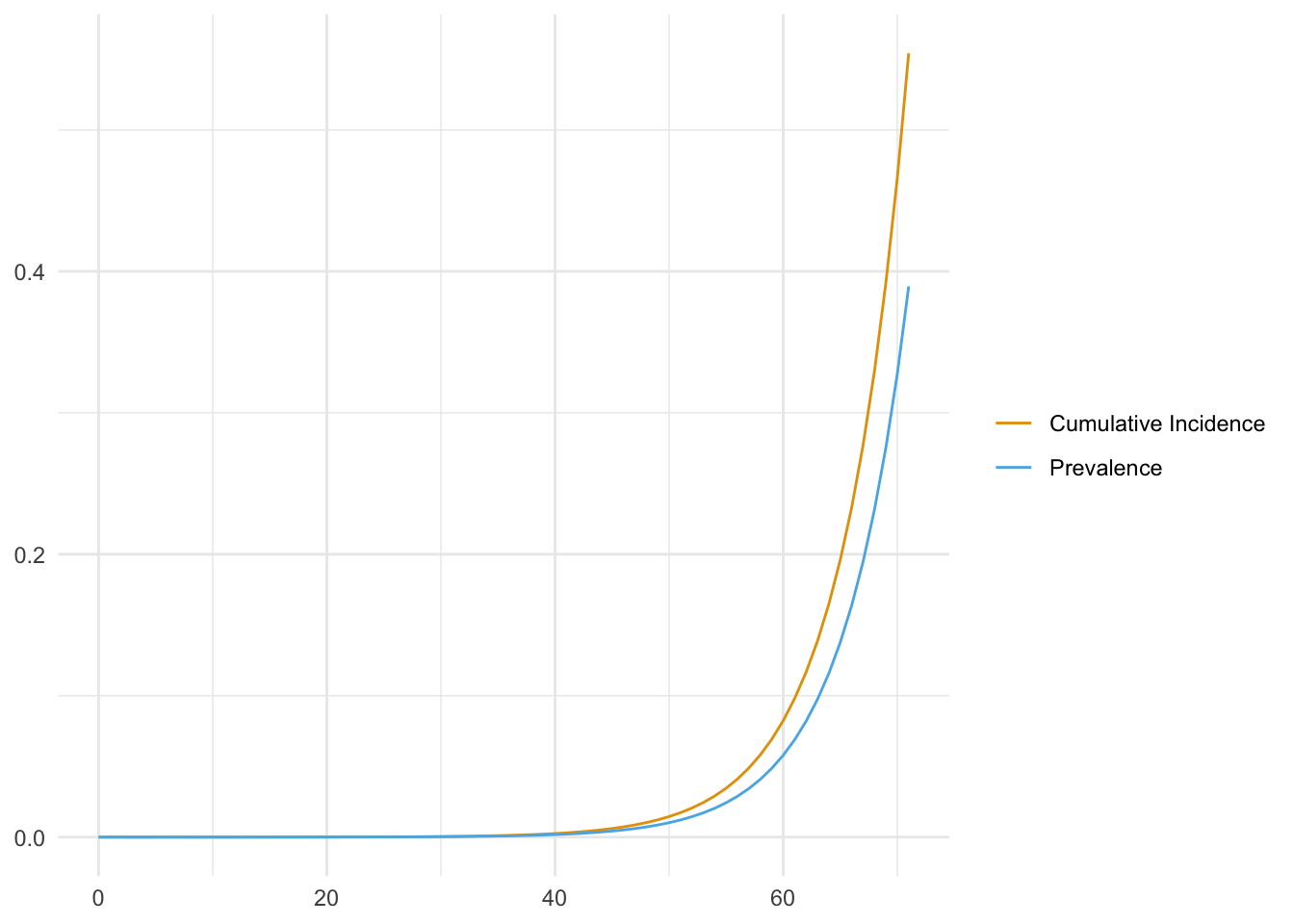

Sampling and sequencing

We assume that the wastewater and pooled nasal swabs are collected every day, and that each sample is sequenced to a constant number of total reads, which differs between swabs and wastewater.
The fitted model predicts the number of reads that are assigned to the whole genome. Here, we are interested in the number of reads that overlap the junction. To predict the number of junction-covering reads, we assume that each read assigned to the genome has an equal probability of overlapping the junction. In our model, this thinning process is equivalent to multiplying the mean number of reads by this probability. For each sample type, we assume that all reads are the same length and that expected coverage is even along the genome. To cover a junction, we require a read to overlap the junction point by a certain number of bases. With these assumptions, probability of covering the junction is equal to the read length minus the required overlap divided by the genome length.
We assume that a junction is detected when reads covering it are observed in two different samples.

# TODO: implement sampling interval. Currently implicitly daily
# sampling_interval <- 1

swab_pool_size <- 300
total_reads_swab <- 2e6
total_reads_ww <- 3e9

# All lengths in bp
read_length_swab <- 2000
read_length_ww <- 170
# To observe a junction, require 15bp on either side
overlap_required <- 30

taxa <- tribble(
   ~species, ~taxid, ~genome_length,
    "Rhinovirus A", 147711L, 7200L,
    "Rhinovirus B", 147712L, 7200L,
    "Rhinovirus C", 463676L, 7100L,
    "HCoV-229E", 11137L, 27500L,
    "HCoV-OC43", 31631L, 30000L,
    "HCoV-NL63", 277944L, 27500L,
    "HCoV-HKU1", 290028L, 30000L,
    "SARS-CoV-2", 2697049L, 30000L
  ) %>%
  mutate(
    # Probability that a read covers the junction, assuming even coverage
    pr_junction_swab = (read_length_swab - overlap_required) / genome_length,
    pr_junction_ww = (read_length_ww - overlap_required)/ genome_length,
  )


# Number of samples required to detect a junction
detection_samples <- 2

Simulations

For model and parameter definitions, see the appendix to our blog post.

First, we load our posterior samples from the swab-p2ra blog post repo. Then, we filter and downsample them in three ways:

We take only the Rhinoviruses and Coronaviruses, the viruses for which we had enough of both swab and wastewater reads to get decent parameter estimates.
We keep the read-model parameters: \(\mu_{swab}\), \(\phi_{swab}\), \(\mu_{ww}\), and \(\phi_{ww}\). (We don’t need the estimates of the prevalence in the Boston samples since our simulations provide the prevalence of the virus.)
To speed up experimentation, for each virus, we randomly downsample the posterior draws.

n_samples = 2000

posteriors <- read_tsv(
  "https://raw.githubusercontent.com/naobservatory/swab-based-p2ra/refs/heads/main/tables/posteriors.tsv",
  show_col_types = FALSE,
  )

thinned_posteriors <- posteriors %>%
  filter(group %in% c("Rhinoviruses", "Coronaviruses (seasonal)", "Coronaviruses (SARS-CoV-2)")) %>%
  select(species, group, mu_swab, phi_swab, mu_ww, phi_ww) %>%
  group_by(species, group) %>%
  slice_sample(n = n_samples) %>%
  mutate(rep = row_number()) %>%
  left_join(taxa, by = join_by(species))

Next, for each virus and for each replicate (posterior draw), we simulate the wastewater and swab reads according to the model. We then summarize each replicate by the cumulative incidence at detection for each sample type.

detection <- thinned_posteriors %>%
  cross_join(epi_model) %>%
  group_by(rep, .add = TRUE) %>%
  mutate(
    mean_ww = prevalence * mu_ww * total_reads_ww * pr_junction_ww,
    reads_ww = rnbinom(n(), size = phi_ww, mu = mean_ww),
    cum_samples_ww = cumsum(reads_ww > 0),
    # Number of swabs from infected people
    pos_swabs = rbinom(n(), size = swab_pool_size, prob = prevalence),
    mean_swab = (pos_swabs / swab_pool_size) * mu_swab * total_reads_swab * pr_junction_swab,
    # Use a finite overdispersion when size and mu are both zero
    # avoids generating NaNs. Should always give zero.
    reads_swab = rnbinom(n(), size = pmax(phi_swab * pos_swabs, 1e-10), mu = mean_swab),
    cum_samples_swab = cumsum(reads_swab > 0),
  ) %>%
  summarize(
    mu_ww = first(mu_ww),
    phi_ww = first(phi_ww),
    mu_swab = first(mu_swab),
    phi_swab = first(phi_swab),
    # If undetected, use 100% CI
    ci_at_detection_ww = if_else(
      any(cum_samples_ww >= detection_samples),
      cumulative_incidence[which.max(cum_samples_ww >= detection_samples)],
      1.0
    ),
    ci_at_detection_swab = if_else(
      any(cum_samples_swab >= detection_samples),
      cumulative_incidence[which.max(cum_samples_swab >= detection_samples)],
      1.0
    ),
    .groups = "drop_last",
  )

In some replicates, a method does not detect the virus by the end of the simulations. In these cases, the cumulative incidence at detection is between 50% and 100%, and we record it as 100%. How often does this happen?

detection %>%
  summarize(
    swab = sum(ci_at_detection_swab > 0.99),
    wastewater = sum(ci_at_detection_ww > 0.99),
    .groups = "drop",
  ) %>%
  select(-group) %>%
  kable

Number of replicates (out of 2000) where the virus is not detected by 50% cumulative incidence
species	swab	wastewater
HCoV-229E	0	1
HCoV-HKU1	1	244
HCoV-NL63	0	60
HCoV-OC43	0	2
Rhinovirus A	0	7
Rhinovirus B	0	20
Rhinovirus C	0	0
SARS-CoV-2	1	0

It is very rare to fail to detect in swabs, but happens as often as 12% of the time in wastewater (HCoV-HKU1).

Results

Below are the results of our simulations. Note that all the values here are conditional on the parameters defined in the Model section. If we change the pool sizes, sequencing depths, read lengths, etc, the comparisons will change.

First, we summarize the simulations with the geometric mean cumulative incidence at detection for each virus and sample type:

geom_means <- detection %>%
  summarize(
    ci_at_detection_ww = gm(ci_at_detection_ww),
    ci_at_detection_swab = gm(ci_at_detection_swab),
    ratio = ci_at_detection_ww / ci_at_detection_swab,
    .groups = "drop",
  )

geom_means %>%
  select(- group) %>%
  rename(
    wastewater = ci_at_detection_ww,
    swab = ci_at_detection_swab,
  ) %>%
  kable(digits = c(NA, 5, 5, 2)) %>%
  column_spec(c(2, 3, 4), width = "3cm", monospace = TRUE)

Geometric mean cumulative incidence at detection. Ratio is wastewater CI / swab CI. Ratio < 1 means earlier detection in wastewater; ratio > 1 means earlier detection in swabs.
species	wastewater	swab	ratio
HCoV-229E	0.01766	0.00194	9.10
HCoV-HKU1	0.11313	0.00721	15.69
HCoV-NL63	0.07759	0.01352	5.74
HCoV-OC43	0.02934	0.00783	3.75
Rhinovirus A	0.02675	0.01067	2.51
Rhinovirus B	0.03617	0.00472	7.67
Rhinovirus C	0.00453	0.00346	1.31
SARS-CoV-2	0.00039	0.00341	0.11

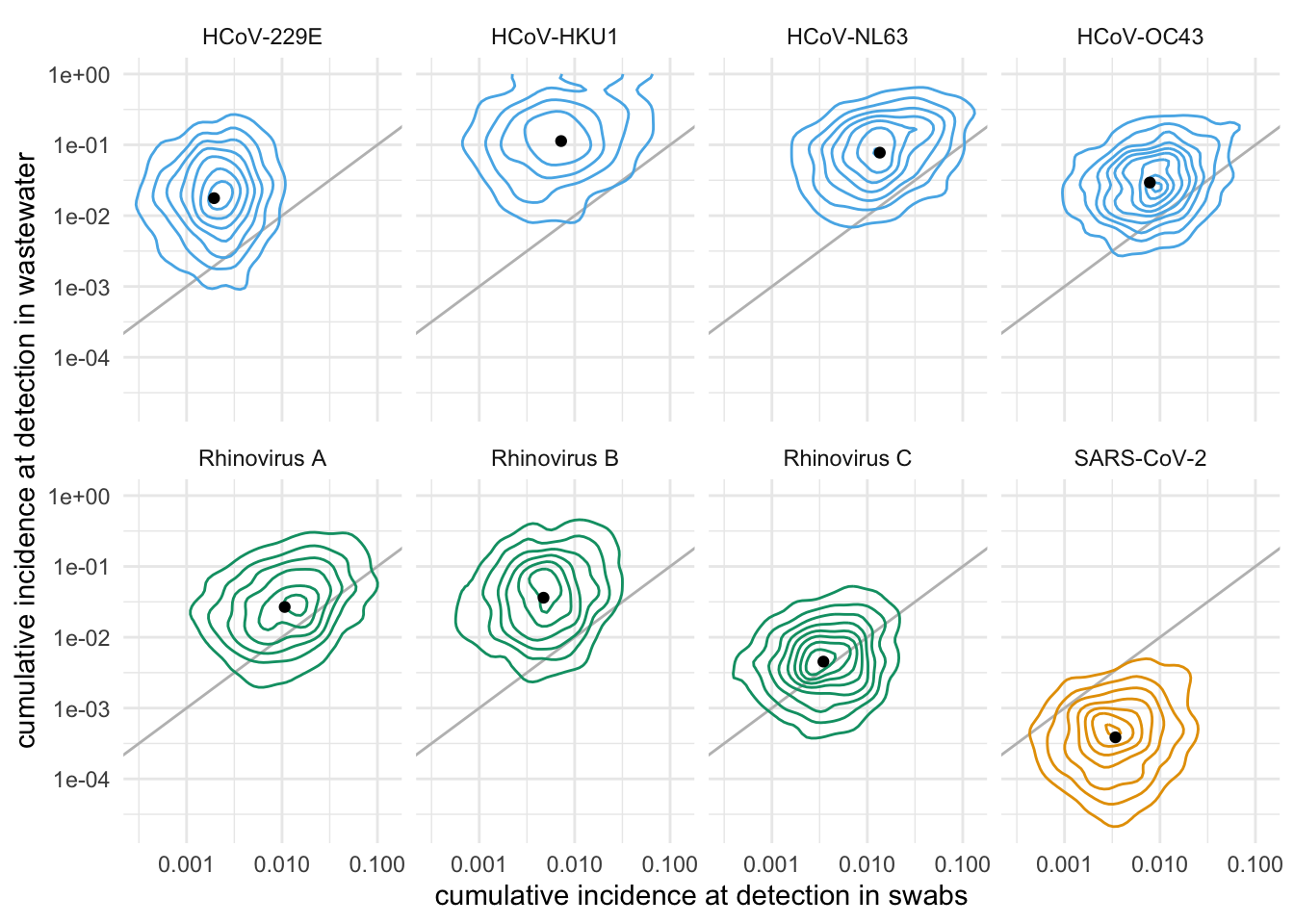
We can also plot the full joint distributions of cumulative incidence at detection:

detection %>%
  ggplot(aes(ci_at_detection_swab, ci_at_detection_ww, color = group)) +
  geom_abline(intercept = 0, slope = 1, color = "grey") +
  geom_density_2d() +
  geom_point(data = geom_means, color = "black") +
  scale_x_log10() +
  scale_y_log10() +
  facet_wrap(~species, nrow = 2) +
  theme(legend.position = "none") +
  labs(
    x = "cumulative incidence at detection in swabs",
    y = "cumulative incidence at detection in wastewater",
    )

Cumulative incidence at detection: wastewater vs. swab. Black dot show geometric means. Grey line is equal incidence. Points above the grey line indicate earlier detection in swabs and vice versa.

Finally, we can plot the distribution of the ratio of CI at detection in the two methods:

detection %>%
  mutate(ratio = ci_at_detection_ww / ci_at_detection_swab) %>%
  ggplot(aes(ratio, species, fill = group)) +
  geom_vline(xintercept = 1, color = "darkgrey") +
  geom_violin(draw_quantiles = c(0.15, 0.5, 0.85)) +
  scale_x_continuous(
    transform = "log10",
    labels = scientific,
    breaks = c(1e-2, 1, 1e2)
    ) +
  theme(legend.position = "none") +
  labs(x = NULL, y = NULL)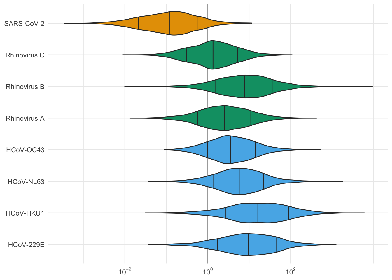

**Ratio of cumulative incidence at detection in wastewater vs swabs** . Vertical bars are 15, 50, and 85th percentiles. Ratio < 1 means earlier detection in wastewater; ratio > 1 means earlier detection in swabs.

These simulations show that, with these sampling and sequencing parameters, for most of these viruses, we expect detection in swabs at 1.3 to 15 times lower cumulative incidence than in wastewater. The big exception is SARS-CoV-2, which sheds a lot in wastewater, for which the simulations suggest 10x lower relative abundance at detection in wastewater than in swabs.

A major caveat is that we are not modeling the delay between sample collection and detection. With exponential growth, delay can be very costly in terms of cumulative incidence. With the 4-day doubling time assumed here, a two-day delay results in a 1.4-fold increase in the cumulative incidence at detection.

Heuristic analysis

We’d like to sanity check and try to understand our simulations with a simpler heuristic calculation. This analysis leaves out a lot of details, but it should be a reasonable rough check.

Leaving aside randomness in read counts and the details of sampling and detection, a simple way to compare the methods is the prevalence at which we expect to see at least one read covering the junction. We’ll call this prevalence \(p^*\). With exponential growth, prevalence is roughly proportional to cumulative incidence, so the ratio \(p^*_{ww} / p^*_{swab}\) is a proxy for the ratio of cumulative incidences at detection in wastewater vs swabs.

For wastewater, the condition to see one read covering the junction is: \[ p^*_{ww} \times \mu_{ww} \times \text{total reads} \times \text{Pr\{read covers junction\}} = 1. \]

For swabs, the condition depends on the pool size. For small pools, the limiting factor is getting a swab from an infected person. For large pools, the limiting factor is sequencing deeply enough to observe reads from the infected swabs. Together, the condition to see one read covering the junction is: \[ p^*_{swab} \times \min(\text{pool size}, \mu_{swab} \times \text{total reads} \times \text{Pr\{read covers junction\}}) = 1. \] Equivalently, we can think of two regimes depending on whether the expected number of junction-covering reads per infected swab: \[ \frac{\mu_{swab} \times \text{total reads} \times \text{Pr\{read covers junction\}}}{\text{pool size}} \] is greater than or equal to one.

We can calculate these heuristics with our parameters:

heuristics <- thinned_posteriors %>%
  mutate(
    prev_ww = 1 / (mu_ww * total_reads_ww * pr_junction_ww),
    prev_swab = 1 / pmin(swab_pool_size, mu_swab * total_reads_swab * pr_junction_swab),
    reads_per_infected_swab = mu_swab * pr_junction_swab * total_reads_swab / swab_pool_size,
    # Because prevalence and cumulative incidence are proportional for exponential
    # growth, we can use the ratio of prevalences to estimate the ratio of CI
    ratio = prev_ww / prev_swab,
  ) %>%
  summarize(
    across(c(reads_per_infected_swab, ratio), gm),
    .groups = "drop"
  )

left_join(
  select(heuristics, species, reads_per_infected_swab, ratio),
  select(geom_means, species, ratio),
  by = join_by(species),
  suffix = c(".heuristic", ".simulation")
) %>%
  rename(heuristic = "ratio.heuristic", simulation = "ratio.simulation") %>%
  kable(digits = c(NA, 2, 2, 2)) %>%
  column_spec(c(2, 3, 4), width = "3cm", monospace = TRUE)

Ratio of cumulative incidence at detection in wastewater to swabs
species	reads_per_infected_swab	heuristic	simulation
HCoV-229E	113.39	12.26	9.10
HCoV-HKU1	0.69	27.48	15.69
HCoV-NL63	0.15	8.08	5.74
HCoV-OC43	0.38	7.23	3.75
Rhinovirus A	0.21	3.49	2.51
Rhinovirus B	1.15	14.24	7.67
Rhinovirus C	1.63	2.65	1.31
SARS-CoV-2	4.08	0.22	0.11

The heuristics and simulations broadly agree, with the heuristic being roughly two times more favorable to swabs than the simulations. This suggests that the noise that our heuristic neglects hurts the efficacy of swabs.